# QUBO NN - Redundancy in QUBOs and finding different representations by making qbsolv differentiable
QUBO-NN, the at this point rather large QC project I've been working on, has enjoyed some interesting updates, which I'd like to share here.
The previous post from April this year can be found here. In that post I described the general idea of reverse-engineering QUBO matrices and showed some preliminary results. The gist of that is as follows: Classification works really well, i.e. at that point classifying between 11 problems showed very high accuracy above 99.8%, while reverse-engineering (the following regression task: QUBO -> original problem, e.g. the TSP graph underlying a given TSP QUBO) is a bit more split. In the following table it can be seen that mostly graph-based problems are easily reverse-engineered (the +), while others such as Set Packing or Quadratic Knapsack cannot be fully reverse-engineered. Note that this table is directly from the Github project.
| Problem | Reversibility | Comment |
|---|---|---|
| Graph Coloring | + | Adjacency matrix found in QUBO. |
| Maximum 2-SAT | ? | Very complex to learn, but possible? C.f. m2sat_to_bip.py in contrib. |
| Maximum 3-SAT | ? | Very complex to learn, but possible? |
| Maximum Cut | + | Adjacency matrix found in QUBO. |
| Minimum Vertex Cover | + | Adjacency matrix found in QUBO. |
| Number Partitioning | + | Easy, create equation system from the upper triangular part of the matrix (triu). |
| Quadratic Assignment | + | Over-determined linear system of equations -> solvable. P does not act as salt. A bit complex to learn. |
| Quadratic Knapsack | - | Budgets can be deduced easily (Find argmin in first row. This column contains all the budgets.). P acts as a salt -> thus not reversible. |
| Set Packing | - | Multiple problem instances lead to the same QUBO. |
| Set Partitioning | - | Multiple problem instances lead to the same QUBO. |
| Traveling Salesman | + | Find a quadrant with non-zero entries (w/ an identical diagonal), transpose, the entries are the distance matrix. Norm result to between 0 and 1. |
| Graph Isomorphism | + | Adjacency matrix found in QUBO. |
| Sub-Graph Isomorphism | + | Adjacency matrix found in QUBO. |
| Maximum Clique | + | Adjacency matrix found in QUBO. |
It should be noted though that there is still some variance in the data (judging by the values being far above ) that can be explained by the models I trained. Thus, while the table says that 5 problems are not reversible, for example of the data is still reversed by the model, which is not bad. The details of the exact reversibility will either be published in a paper or are available by contacting me, since this is too much for this blog post. This also includes 3 more problem types (Graph Isomorphism, Sub-Graph Isomorphism and Maximum Clique), bringing the total to 14 supported problem types. The very nice t-SNE plot for the classification is seen next.
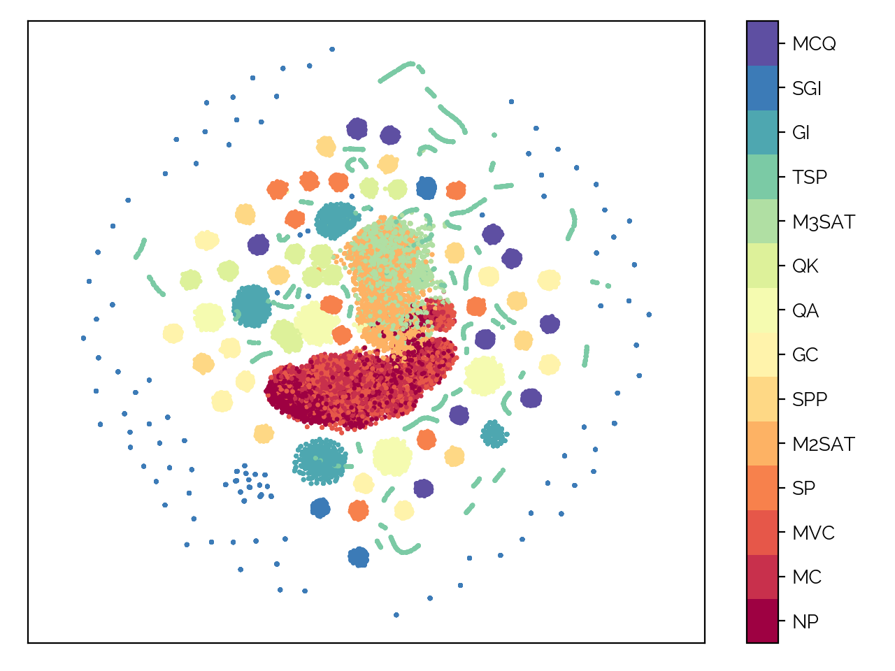
Due to supporting the translation of 14 problem types into QUBOs, I've decided to publish the project as a package on pypi. There are likely more problem types coming up that will be supported as well, thus this package may become useful for others in the industry. The exact list of problems implemented is:
- Number Partitioning (NP)
- Maximum Cut (MC)
- Minimum Vertex Cover (MVC)
- Set Packing (SP)
- Maximum 2-SAT (M2SAT)
- Set Partitioning (SP)
- Graph Coloring (GC)
- Quadratic Assignment (QA)
- Quadratic Knapsack (QK)
- Maximum 3-SAT (M3SAT)
- Traveling Salesman (TSP)
- Graph Isomorphism (GI)
- Sub-Graph Isomorphism (SGI)
- Maximum Clique (MCQ)
Now, a few more things were investigated: First of all, the classification and reverse-engineering was extended to a more generalized dataset which does not contain just one problem size (and thus one QUBO size), but multiple, which are then zero-padded. So for instance, a dataset consisting of QUBO matrices could also contain zero-padded QUBOs of size or . This worked really well, though some problem types (mostly the ones that scale in ) required more nodes in the neural network to reach the same and thus the same model performance, since the model had to differentiate between the different problem sizes in the dataset.
Further, the general redundancy in QUBOs was studied: AutoEncoders were trained for each problem with differing hidden layer sizes, and the resulting when reconstructing the input QUBO was saved. A summary of the data is seen in the figure below.
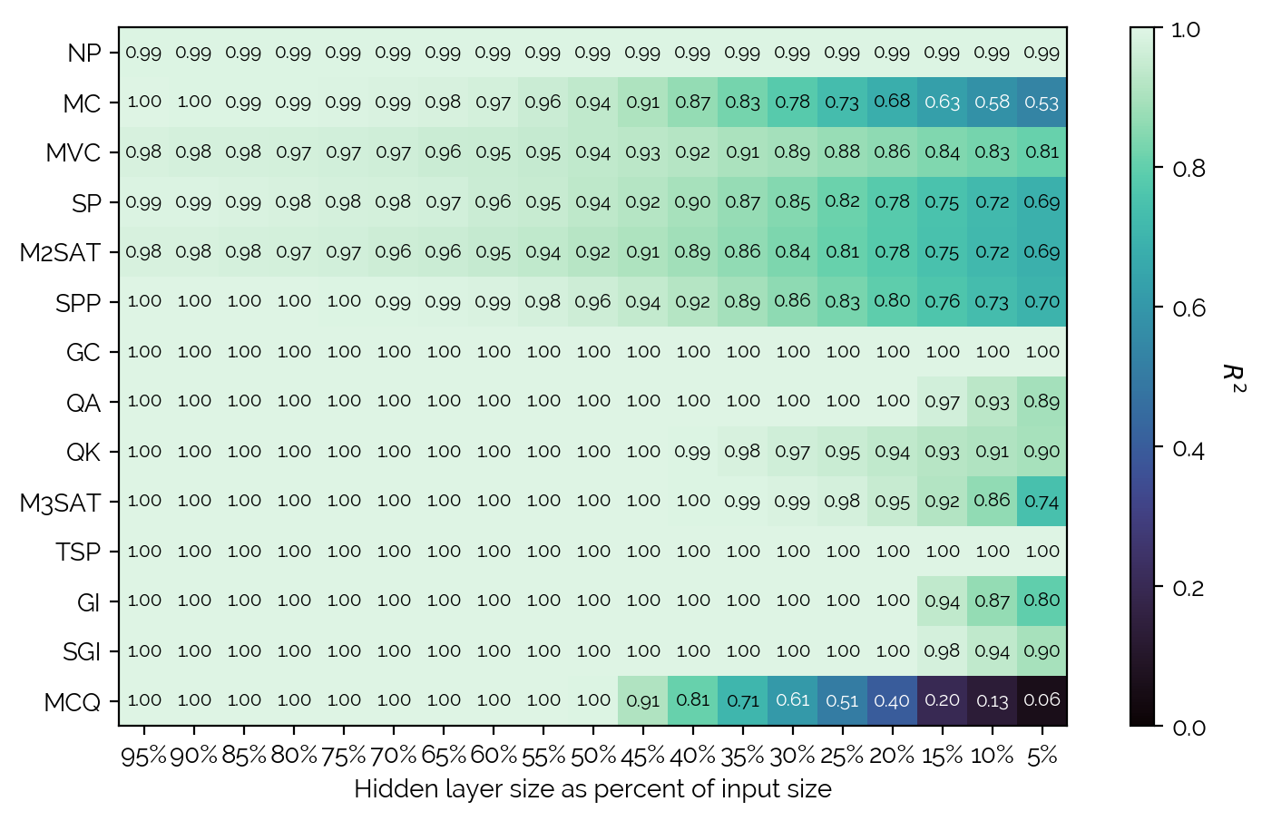
Doing a step-back, it can be seen that there is in general a lot of redundancy. There are also some interesting differences between the problem types in terms of how much redundancy there is - for instance, TSP or GC have so much redundancy that even a hidden layer size of 204 (from the input size of 4096) is enough to completely reconstruct the QUBO. Mostly the QUBOs that scale in and QUBOs that in general have a very lossy translation. It is surprising that graph-based problems that have an adjacency matrix do not allow much compression and thus do not have as much redundancy (cf. Maximum Cut or Minimum Vertex Cover).
The project also includes a lot of attempts at breaking classification. The goal here is to find a different representation of the QUBOs that is extremely similar (so all the QUBOs are similar) while making sure they still encode the underlying problem and represent valid QUBOs. For this, the following AutoEncoder architecture (shown for 3 problem types, but easily extendable to more) was used.

It includes reconstruction losses, a similarity loss (just MSE) between the hidden representations and a qbsolv loss (not shown) that ensures that the hidden representations are valid QUBOs (which otherwise would not be the case, and which makes this whole exercise void). The qbsolv loss is based on a special layer as proposed in Vlastelica et al., and the exact implementation in QUBO-NN can be found here.
This wraps up this post for now - of course there is still a lot more to discuss, but this is for another post. Check out the Github repository if you are interested.
References:
- Vlastelica et al., "Differentiation of Blackbox Combinatorial Solvers"