Filling a docx template with Python while preserving style

# Filling a docx template with Python while preserving style

I am actually amazed how easy this is - check the example below. There are a few gotchas to keep track of, but all in all - very easy.

A common issue arises with placeholders in a Word document – they might be split into multiple runs. A run in Word is a region of text with the same formatting. When editing a document, Word may split text into multiple runs even if the text appears continuous. This behavior can lead to difficulties when replacing placeholders programmatically, as part of the placeholder might be in one run, and the rest in another. To avoid this, it's crucial to ensure that each placeholder is written out in one go in the Word document before saving it. This step ensures that Word treats each placeholder as a single unit, making it easier to replace it programmatically without disturbing the rest of the formatting.

Here’s how you can automate the replacement of placeholders in a Word document while preserving the original style and formatting. This approach is particularly useful for generating documents like confirmation letters, where maintaining the professional appearance of the document is crucial.

from docx import Document

# Function to replace text without changing style
def replace_text_preserve_style(paragraph, key, value):
    if key in paragraph.text:
        inline = paragraph.runs
        for i in range(len(inline)):
            if key in inline[i].text:
                text = inline[i].text.replace(key, value)
                inline[i].text = text

# Load your document
doc = Document('path_to_your_document.docx')

# Mock data for placeholders
mock_data = {
    "PLACEHOLDER1": "replacement text",
    "PLACEHOLDER2": "another piece of text"
    # Add as many placeholders as needed
}

# Replace placeholders with mock data
for paragraph in doc.paragraphs:
    for key in mock_data:
        replace_text_preserve_style(paragraph, key, mock_data[key])

# Save the modified document
doc.save('path_to_modified_document.docx')

In this script, replace_text_preserve_style is a function specifically designed to replace text without altering the style of the text. It iterates through all runs in a paragraph and replaces the placeholder text while keeping the style intact. This method ensures that the formatting of the document, including font type, size, and other attributes, remains unchanged.

When preparing your template, make sure each placeholder is inserted as a whole (this means - go into the template and write the placeholders in one go, then save the docx). Avoid breaking it into separate parts, or only writing a part of the placeholder. Word needs to consider the whole placeholder as one unit. This preparation makes it easier for the script to find and replace placeholders without messing with the document’s formatting.

This approach is incredibly effective for automating document generation while maintaining a high standard of presentation. It's particularly useful in business contexts where documents need to be generated rapidly but also require a professional appearance. We use this a lot at rhome to automate all kinds of registration documents.

Published on 2024-01-21

# Reliable structured extraction of descriptions with GPT and Pydantic

Diving straight into the the matter, we're looking at a high-powered, AI-driven approach to extracting technology requirements from project descriptions. This method is particularly potent in the fast-paced freelance IT market, where pinpointing exact requirements quickly can make or break your success. Here’s how it’s done.

Firstly, let’s talk about Pydantic. It’s the backbone of structuring the sometimes erratic outputs from GPT. Pydantic's role is akin to a translator, making sense of what GPT spits out, regardless of its initial structure. This is crucial because, let's face it, GPT can be a bit of a wildcard.

Consider this Pydantic model:

from pydantic import BaseModel, Field

class Requirements(BaseModel):
    names: list[str] = Field(
        ..., 
        description="Technological requirements from the job description."
    )

It’s straightforward yet powerful. It ensures that whatever GPT-4 returns, we mold it into a structured format – a list of strings, each string being a specific technology requirement.

Now, onto the exciting part – interfacing with GPT-4. This is where we extract the gold from the mine.

import openai

class RequirementExtractor:
    def __init__(self, project_id: int):
        ...
        self.project: Project = Project.query.get(project_id)
        self.openai_client = openai.OpenAI(api_key=os.environ.get("OPENAI_API_KEY"))

    def _extract_requirements(self, description: str) -> Requirements:
        ...

In this snippet, the RequirementExtractor initializes with a project object. The real action happens in _extract_requirements. This method calls upon GPT-4 to analyze the project description and extract technology requirements.

The extraction process is where things get interesting. It's not just about firing off a request to GPT-4 and calling it a day. There's an art to it.

def _extract_requirements(self, description: str) -> Requirements:
    response = self.openai_client.chat.completions.create(
        model="gpt-4",
        response_model=Requirements,
        messages=[
            {"role": "system", "content": "Extract technology requirements."},
            {"role": "user", "content": description}
        ],
    )
    return response

We send the project description to GPT-4 with a specific prompt to extract technology requirements. It’s precise and to the point. The response is then funneled through our Pydantic model to keep it structured.

Accuracy is key, and that’s where iterative refinement comes in. We don't settle for the first output. We iterate to refine and ensure comprehensiveness.

def extract(self) -> list[str]:
    ...
    while retries_left > 0 and total_retries < self.MAX_RETRIES:
        response = self._extract_requirements(self.project.description)
        ...
        total_retries += 1
    ...

This loop keeps the process going, refining and adjusting until we have a complete and accurate set of requirements.

The final touch is grouping similar technologies. It’s about making sense of the list we’ve got, organizing it into clusters for easier interpretation and application.

def group(self, requirements: list[str]) -> GroupedRequirements:
    ...
    return self.openai_client.chat.completions.create(
        model="gpt-4",
        response_model=GroupedRequirements,
        messages=[
            ...
        ],
    )

In this function, we again leverage GPT-4’s prowess, but this time to group similar technologies, adding an extra layer of organization to our extracted data.

In the German freelance IT market, speed and precision are paramount. Imagine applying this method to a project posting for a Senior Fullstack Developer. You get an accurate, well-structured list of requirements like AWS, React, and domain-driven design in minutes. This is crucial for staying ahead in a market where projects are grabbed as soon as they appear.

Harnessing GPT and Pydantic for requirement extraction is more than a convenience – it’s a strategic advantage. It’s about extracting the right info, structuring it for practical use, and doing it all at lightning speed. This approach isn’t just smart; it’s essential for anyone looking to dominate in the competitive, fast-paced world of IT freelancing.

Published on 2024-01-20

# Ode to capitalism

The Role of Capitalism in Addressing Contemporary Challenges

This perspective examines the current challenges facing humanity as opportunities for growth and innovation, akin to past historical instances such as the World Wars. It contends that despite the prevalent challenges, capitalism remains an efficient solution. Optimistic figures like Warren Buffett have reaped rewards during such turbulent times. The Product-Market Fit (PMF) process in building startups is instrumental in selecting businesses that create value, while others naturally fade. Capitalism, due to its incentive structure, continues to be a powerful driver of innovation. Despite human selfishness, it fosters collaboration. In contrast, a shift to communism or a full welfare state may diminish personal motivation. The resolution of issues in these systems typically relies on voluntary effort. Some government intervention can provide an impetus, but the majority should be left to the free market and capitalism.

Regarding the concept of endless growth, it's intriguing to note the correlation between dire predictions and population growth in recent decades. The outlook suggests a deceleration in GDP growth in OECD countries, and consumer saturation prevails. This pattern illustrates a reversed "S" curve, characterized by exponential growth followed by a plateau. While China, India, and Africa currently propel global growth, even their population growth forecasts have been adjusted downward due to faster wealth accumulation. This adjustment signals their eventual transition into a phase of diminishing growth (Saunders, 2016).

A recent study by the OECD supports this assertion, highlighting a trend of declining resource consumption in OECD countries. "The materials intensity of the global economy is projected to decline more rapidly than in recent decades — at a rate of 1.3% per year on average — reflecting a relative decoupling: global materials use increases, but not as fast as GDP" (OECD, 2008, 2018, 2020).

While capitalism presents its own set of challenges and is far from perfect, it continues to exhibit adaptability and innovation. It does not inherently drive infinite exponential growth. However, there is substantial cause for optimism, as humanity has historically overcome challenges. Hence, I remain fully invested in stocks, confident in our ability to navigate the future.

References:

Saunders, H. (2016). "Does Capitalism Require Endless Growth?". Retrieved from https://thebreakthrough.org/journal/issue-6/does-capitalism-require-endless-growth

OECD. (2020). Toward a More Resource-Efficient and Circular Economy. Retrieved from https://www.oecd.org/environment/waste/OECD-G20-Towards-a-more-Resource-Efficient-and-Circular-Economy.pdf

OECD. (2018). Global Material Resources Outlook to 2060. Retrieved from https://www.oecd.org/environment/waste/highlights-global-material-resources-outlook-to-2060.pdf

OECD. (2008). Waste Management and Circular Economy in OECD-G20 Countries. Retrieved from https://www.oecd.org/environment/waste/47944428.pdf

Published on 2023-10-14

# Rapid MVP development with figma code export plugins

This is just a short trick I'd like to share. I've built countless of MVPs, some paid, some as a cofounder, some as a friend service. Over time I've started to optimize the process. Sometimes there is a given design in Figma. This is a perfect case, since we can use plugins to export code that gives us a great basis to continue from.

I've tested a multitude of plugins, the one that worked best so far is the "Figma to HTML"-plugin by Storybrain. Find the Figma plugin here.

The concrete steps to quickly build an MVP from a Figma design:

Autolayout -> if the design is built well, this will already be no issue. If it is not, you will have to go through all logical groups (horizontal and vertical) and "group" them with autolayout.
Use the plugin to export to React.
Fix up small issues (but you won't have to..), make it responsive if needed.
Build the backend (use supabase here for rapid development).
Connect backend to frontend, add basic login/signup and CRUD functionality. This is the most manual step that I have not found a way around so far.
Profit.

This process enables us to build MVPs of platforms and SaaS solutions based on a given design in basically one day. It also enables us to continue work. Especially with the plugin by Storybrain the quality is usually good enough to get as far as seed stage in my opinion.

There are a couple of drawbacks:

The CSS is mostly duplicate. I have no solution here as of yet, but I am sure there are ways.
Garbage in, garbage out - if the Figma design is built in a bad way (bad naming conventions, bad grouping), the resulting code will contain these as well.

Lastly, is there a business risk by relying on one random free Figma plugin? Yes, of course. There are others that work nearly as well however. Check out FigAct for example.

Published on 2023-06-10

# Leaked list of 1923 SEO factors of yandex search

SEO has always been mainly characterized by the arms race between search engine providers such as Google or Yandex and SEO specialists. Well, today has been quite an amazing day for public SEO - a large amount of the source code of Yandex was leaked, which includes amongst others a list of 1923 search engine factors / SEO factors.

Since in the original source code the descriptions are all in Russian, I've translated them to English (note, I did not go through all 1923 factors, there could be some translation errors).

You can find the list of 1923 factors here.

I find a few of them quite interesting.

1/ Notably there are quite a lot of checks across basically everything the host can give to find whether the site could be spam - this includes checking whois information, the site realiablity (i.e., how many 400/500 errors the site has),

2/ There is also a large group of user behavior related checks, such as how long a user visited the site, what they clicked, basically the whole user journey. Look for "entropy"-related factors in the list of factors that I shared, those are all related to how the user behaves statistically. This also includes how "rapid" the user clicks, which I find quite interesting.

3/ There are also some super naive looking (but likely effective against spam, else they wouldn't be included) checks such as how many slashes the URL contains, or whether there are any digits, or whether certain specific phrases are contained, that I won't quote here since I would be impacting this blog negatively lol.

4/ Site types: There are factors whether the site is a blog/forum, shop, news, etc., or whether it is related to law and finance.

5/ Wikipedia is also boosted specifically, and TikTok has its own factor.

6/ One major factor (or list of factors) is how natural the text reads, or how "nasty" it is (literally called the "nasty content factor").

7/ There are a lot of factors related to geography, e.g. matching the language of the user that is visiting the link has impact. Or the distance of the request to the city Magadan or Ankara. Huh?

8/ There are factors related to having a playable video on the page and having downloadable files (including videos).

9/ Looking at the war between Russia and Ukraine - there are also factors indicating whether the site is in Russian or Ukrainian.

10/ SUPER interesting: "Url is a channel/post from a verified social network account" -> makes sense of course, but having a verified social media account refer to a URL could be a boost on par with having a nice backlink.

11/ And lastly, of course, there are standard SEO factors that include PageRank, backlinks, Trust Ratio (TR), BM25, and so on..

Check out the list yourself - ping me if you have awesome insights to include in this post.

Published on 2023-01-28

# Bypassing certificate pinning without root using frida gadget

An unusual post again, but quite the adventure that I had to share. As a kid I used to venture into exploits and hacking. I've rekindled the old days and looked into a mobile app more deeply. To make sure I don't incriminate myself I won't mention the app, the main tech stack is as follows though - the app basically has a list of users that can be listed in a very slow manner (shows like 10 users and swiping+loading the next batch is super slow). The app talks with multiple backend services such as Firebase etc., but most importantly uses Algolia search. My goal was to get all users.

First, what I tried.

1/ Start simple: Get a network monitor such as "PCAPdroid" or "PCAP remote" directly on my phone (both good ones btw - I tried some more, those two are good). The goal was to understand more what kind of backend calls are made from the app. These kind of apps also allow injecting a self-signed certificate via a VPN to decrypt the HTTPS/SSL calls - but here I learned something new. Apparently mobile security has advanced and now in every state of the art app there exists this concept of public key pinning or certificate pinning. Won't go too deep into that, but it's basically a whitelist of certificates hard-coded into the app in some way or another, which means a self-signed certificate won't be accepted by the app.

2/ Next step was clear - I needed to decompile the app and take a deeper look. So I did just that. I installed apktool via brew install apktool and ran:

apktool d app

This results in smali files, which is the assembly language used by the Android system. Here I will shorten my adventure, since I now wasted a few hours trying to bypass the certificate pinning by trying to modify the internal files and smali code of the app by hand. In the end I likely simply missed something, since I did not get it to work. To be fair, the app was huge with a large set of external libraries.

To recompile I used the following process on Mac. First of all I had to add Android Studio (and the Python binary directory, but later more on that) to my PATH:

export PATH=/Users/instance/Library/Android/sdk/build-tools/33.0.0/:$PATH
export PATH="/Users/instance/Library/Python/3.10/bin:$PATH"

Next, I used the following commands. Note that zipalign and apksigner come from the build tools directory added above to our PATH. This is very interesting since SO MANY ressources out there are just outdated or don't work. Especially signing with jarsigner is simply a meme - it DOES NOT WORK. At least not on my modern phone with one of the latest Android versions.

apktool b app
cp app/dist/app.apk app2.apk
rm -f app2-aligned.apk
zipalign -v 4 app2.apk app2-aligned.apk
apksigner sign --ks ~/.keystore --ks-key-alias am app2-aligned.apk

So as you can see you first recompile, then do the zipalign, and then use apksigner to sign. It should be noted that the ".keystore" file was generated beforehand. And again, lots of outdated stuff here! Security requirements move over time.

keytool -genkey -v -keystore ~/.keystore -keyalg RSA -keysize 2048 -validity 10000 -alias app

3/ Finally, frida-gadget. I used the following repository to simply include frida-gadget in the apk directly: https://github.com/ksg97031/frida-gadget

I then installed objection, added the Python binary directory to PATH as mentioned before, enabled USB debugging in my phone (somehow this wasn't enabled yet?! As I said, I haven't been doing this kind of stuff in a while..), installed the modified app on my phone and finally ran in my terminal:

objection explore

(after checking adb devices and making sure my phone is recognized)

This requires you to start the modified app beforehand by the way.

I then disabled certificate pinning in the objection terminal:

android sslpinning disable

And finally started PCAPdroid and voilá - decrypted HTTPs requests, including a juicy Algolia API key. The rest is very simple and took like 10 minutes - extracting all the data from Algolia via Python.

Published on 2022-10-12

# Extending supabase with your own backend - its supa easy!

In recent years lowcode solutions and tech services have become increasingly useful in my opinion. Firebase has become an essential of tech MVPs, and now there is a new kid on the block called supabase. Tested it, loved it. Of course, most of the time you need more than a bit of CRUD, so I will show you in this post how to extend supabase with your own backend. It's actually supa easy. (lol)

First off, what is supabase? I'd say in one sentence: supabase is backend as a service. It runs on PostgreSQL, has an extensive online table editor (cf. picture below), logging, backups, replication, and easy file hosting (akin to Amazon S3).

The best part is how easily plug&play their integration is into your frontend. Check out the example below, that is for uploading a file in React. You can also interact in a very SQL-like fashion with the database from React. Can you believe this?!

// Uploading a file
const file = event.target.files[0]
const fileExt = file.name.split('.').pop()
const fileName = `${Math.random()}.${fileExt}`
const filePath = `${fileName}`

let { error: uploadError } = await supabase.storage
  .from('projectavatars')
  .upload(filePath, file)

// Selecting data
let resp = await supabase
  .from('invitedusers')
  .select(`*`)
  .eq('account_group_id', id_)
  .order('id', { ascending: false })

// Upsert :D
let resp = await supabase.from('invitedusers').upsert({
  "id": invitedNames[idx].id,
  "user_email": invitedNames[idx].user_email,
  "account_group_id": resp.data[0].id,
  "role": invitedNames[idx].role
})

One of the coolest features is the large support for authentification (logging in with ALL kinds of socials, check it out below), and again, with extremely easy integration in your frontend. Amazing.

const { user, session, error } = await supabase.auth.signInWithPassword({
  email: email,
  password: password,
});

const { user, session, error } = await supabase.auth.signInWithOAuth({
  provider: 'google',
})

So now onto the main part - extending supabase with your own backend. There are two elements to this as far as I see it. First, interacting with the database in general - thats supa easy. ;)

Go to your project settings, then to the API tab, and copy your project url and key (cf. picture below).

You can then use those (the url and the key) and simply talk with the database, as seen below.

from supabase import Client
from supabase import create_client

supabase = create_client(url, key)
data = supabase.table('accountgroups').select("*").execute()
for item in data:
    ...

The second element is user-authenticated interaction with the database. Say you want to generate an excel sheet for a user, IF they are logged in. How to check? See below. Note that you can get the JWT in the frontend easily, it's a field in your session object (session.access_token). If you want to know how to set this up in React, go to the end of the post.

supabase = create_client(url, key)
supabase.auth.set_auth(access_token=jwt)

# Check if logged in
try:
    supabase.auth.api.get_user(jwt=jwt)
except:
    return {"error": "not logged in"}

This wraps it up for now. I am now an advocate for Flutterflow and supabase! If you want to know more, check out my Flutterflow post.

Getting the session in the frontend.

Here is how this is set up, basically in the router we get the current session and pass it to all our pages that need it. In the login page we directly interact with supabase.auth, and this gets immediately reflected in our router, and thus passed to all pages.

const RouterDOM = () => {
    const [session, setSession] = useState(null)

    useEffect(() => {
      supabase.auth.getSession().then(({ data: { session } }) => {
        setSession(session)
      })

      supabase.auth.onAuthStateChange((_event, session) => {
        setSession(session)
      })
    }, [])

    return (
        <Router>
{!session ? (
            <Switch>
                <Route exact path="/"><Login /></Route>
                <Route exact path="/new"><CreateAccount /></Route>
            </Switch>
) : (
            <Switch>
                <Route exact path="/"><Home session={session} /></Route>
                <Route exact path="/login"><Login /></Route>
                <Route exact path="/new"><CreateAccount /></Route>
                <Route exact path="/home"><Home /></Route>
// ...
            </Switch>
)}
        </Router>
    );
}

We can then use the session object to pass the JWT to the backend like so:

var form = new FormData();
form.append("user_id", session.user.id);
form.append("jwt", session.access_token);

return fetch(IP + 'create', {
  method: 'POST',
  body: form,
  mode: "cors",
  credentials: "include",
}).then((resp) => {
  console.log(resp);
  return resp.json().then((data) => {
    console.log(data)
    return data;
  });
});

Published on 2022-09-22

# A path of success

Have you ever heard this saying "your 10th startup will be a success!" - implying that your 9 previous startups were total failures.

I see that in a completely different light. Maybe I am deluding myself, but in my opinion it is super easy - while the utmost goal is to build something of lasting value and to deliver, additionally I like to go into each project with this notion (btw, I LOVE notion) of doing an experiment, trying to learn something new. Most of the time these experiments emerge after some time (e.g. you start building, and only after a few weeks you notice an AI component that could make sense). Since this is a general concept, it makes me topic-agnostic. It does not matter whether you do QC or AI, if you are experimenting with supabase to increase the speed of MVP development, or you're experimenting with optimizing the collaboration between designers and developers with figma autolayout, or you're simply experimenting with government processes for registering a non-profit. This is why I have such a broad set of topics - the range is from fintech, QC, to a charity (an actual non-profit legal entity), and many more that I would not be able to list. Try experimenting with things like creating a fully remote team from all around the world. How awesome is that?! I love working with people and making them grow - doing this with people from Asia or Africa makes it so much more fun and rewarding (and of course don't forget the economic value). I learn about cultures FIRST HAND, the struggles, the awesome things (the good, the bad and the ugly one might say), and I already plan on visiting some interesting countries simply due to having this connection.

The cool thing is, this keeps motivation up. So yes, I am deluding myself in a way. In the end what matters is getting something off the ground and not learning something new. My main focus in the end is delivering something of value, to be clear.

I come from engineering which is close to natural sciences (due to math), so I've read my fair share of papers and published some myself. I am always venturing in empirical and experimental papers when i work academically, so recently I have come to love this comparison of academic research to startups - you have a certain hypothesis and you test it out by doing interviews, building an MVP and validating it. It's like I am not studying phenomena in Machine Learning or Quantum Computing anymore, but I am now studying people and economics. Mostly people and their desires if I think about it.

As a knowledge worker in computer science I have the privilege to choose my adventure. Due to all these experiments I am starting to be extremely sure on what I'd choose if I had to, again. Where else can you experiment in such a way and create your own path of success?

Ok that was cheesy. The gist of this is - one can build something significant with consulting, in big corp, by doing startups.. for me, it's startups.

Published on 2022-08-14

# Alphalerts got acquired

Last week, Alphalerts got acquired. I founded this last year out of my own need.

Alphalerts has many hidden goodies that I use myself:

sentiment analysis
downloading and parsing SEC Form-4 reports
ETF constituents
live put/call ratio

The acquisition itself was interesting. I put Alphalerts on secondfounder, which itself is run by Arvind (great guy btw), and quickly got >5 requests. I've read about microacquisitions on Hackernews and LinkedIn before, and the trend was always the same - the final sales always happens rather quickly, and in a really focussed and determined way. I can report the same happened here. Mostly slow and uncertain requests, except for one really focussed guy. He squeezed me with millions of questions in one session and wanted to see some code, then asked for a call, and basically bought it all after that call. Quite an amazing collaboration.

We also connected on a personal level, and I must say, I deeply respect that guy for his motivation and his determination. He has a clear plan, and Alphalerts was just part of this. This guy fucks basically.

Big thanks to Arvind and his secondfounder project. Arvind has big plans as well, quite the amazing person.

So there we go, I can now put 1x exit on my LinkedIn profile. And of course put Startup Coach for good measure.

Published on 2022-07-29

# Flutterflow Firebase ElasticSearch - the new lowcode Trifecta for non-technical founders

I have always had kind of mixed feelings about nocode/lowcode. This just changed yesterday. I've been introduced to Flutterflow - and wow. It combines the ease of creating a nocode app with the flexibility and extensibility of code, since it allows exporting your app as Flutter code. It supports integrating the usual suspects (for example Firebase or ElasticSearch), has very extensible 'custom functions' and a flexible query API for connecting and using all kinds of APIs.

I am not getting paid for this. But from on, if I get asked what one should do without having a technical cofounder, I will refer them to Flutterflow. However, I can still see a case for Flutterflow consulting (same as the consulting ecosystem that has come up around webflow) for more advanced use cases. Take Machine Learning for Flutterflow for instance. Let's say you'd like to create an app that in addition includes a few personalized product or content recommendations - perfect case to hire a small-time Flutterflow consultant. Comes up super cheap, you built the app, and the last 20% you leave to a consultant. Since I hear all the time the struggles to find good hands-on technical cofounders, this I could see as the wide-spread future of MVPs.

From the business perspective I also like their "Flutterflow Advocate" role they're currently hiring for. Similarly to webflow they're likely going for the consultancy ecosystem, which I think is a good idea. Let's see whether they're able to capture this heavily contested market.

Published on 2022-07-01

# Aesthetics of Scheduling QUBOs

This post is more of an appreciation post for quantum annealing and its aesthetics (and not much of a scientific one). We do lots of experiments at Aqarios involving a large number of different optimization problems and their QUBO representation. Most of them have one thing in common - the beautiful patterns of certain orders. We humans love patterns so so much. Patterns give us a sense of order. Since order gives predictability, which gives a sense of control, we all deep down love order.

For instance, check out this very interesting series of job shop scheduling QUBOs. From top to bottom, the QUBO sizes vary in 50, 100, 200 and 300.

I won't comment on the patterns itself, but the series is interesting - one can see how increasing the parameter T (which in job shop scheduling controls the strict upper time bound when all jobs should be finished) dilutes the contraints. The next series shows nurse scheduling QUBOs with the same size variation as in the job shop scheduling example.

I'd like to highlight the dilution again. Though, one most note, that the very distinct white diagonals stay in the same position. The last series is one that I find the most amazing. This is satellite scheduling, and especially the lower sizes show this beautiful pattern that reminds me of a light ray.

While this wasn't one of my usual scientific or business related posts, I still think it is nice to sometimes take a step back and just observe the beauty of nature and logic.

My deep thanks goes to our prolific QC expert Michael Lachner for generating those illustrations.

Published on 2022-05-07

# Improving evolutionary algorithms using quantum computing

I love the concept of QAGA - the quantum-assisted genetic algorithm. A standard evolutionary algorithm consists of a recombination phase, a mutation phase, and a selection phase. In the case of QAGA the mutation phase is done using reverse quantum annealing. In the latest research from Aqarios in cooperation with LMU Munich we improved the published QAGA algorithm on a set of problems (Graph Coloring, Knapsack, SAT). Since simulated annealing can be used for reverse annealing as well, we first tested solely on classical compute (we called the algorithm using simulated annealing SAGA), and later went for experiments with quantum compute. Slightly risky, but very effective, this allowed us to test a large number of modifications due to the high cost of QC right now.

We will publish the results in the QC Workshop at GECCO 2022 - I will link the paper soon.

Note that the recombination phase can also be computed with quantum annealing - see my other post here.

Specifically, the following modifications were tested:

Simpler selection (ignoring the shared Ising energy and only using the individual energy)
Simpler recombination (one-point crossover, random crossover) instead of the cluster moves
Incremental sampling size, specifically increasing the number of sweeps and the population size over time
Decreasing annealing temperature over time
Parameter mutation - each individual of the population also includes the annealing temperature, which is thus mutated as well
Multiprocessing
Combinations of the above and further minor modifications (see our publication)

The next Figure shows an overview of the modifications from the paper with shortnames. The shortnames are important to understand further Figures with results.

Next, the first results are shown. It is clear that our crossover modifications work well, and that we find for all problems a modification that improves upon the baseline - though we are not able to find a general improvement on all problems investigated here at the same time. Increasing the number of sweeps and decreasing the annealing temperature also both work very well.

Lastly, the following Figure shows our results on quantum hardware. It is clear that the modifications on SAGA also partly transfer to quantum compute.

Not only does this show that we were able to improve a genetic algorithm (that I would call the strategic micro-scale of this project), but this also shows that it is feasible to do experimentation on classical hardware and transfer the results to quantum compute later.

Super happy about the results - only possible with all the great work by everyone involved!

Published on 2022-05-01

# List of 41 Quantum Computing Stocks and Public Companies

Below I show a list of public quantum computing companies and stocks that anyone with a brokerage account can invest in in 2022. It is quite amazing how much is already out there. The pure QC plays are few as of now, but still - they are growing.

Pure QC plays in the US (Nasdaq/NYSE):

Ticker	Company
ARQQ	Arqit
IONQ	IonQ
QUBT	Quantum Computing Inc
HON	Honeywell
RGTI	Rigetti

Note that this is mostly hardware - QC software companies are still mostly private, since they are still up and coming.

The following shows the usual suspects. While their core business is something else, these companies all invest into QC. Of course, leading tech stocks, semiconductors, but also military defense companies such as Lockheed:

Ticker	Company
GOOG	Google
AMZN	Amazon
IBM	IBM
INTC	Intel
NVDA	Nvidia
MSFT	Microsoft
AMD	AMD
LMT	Lockheed Martin
TSM	Taiwan Semiconductor
AMAT	Applied Materials
ACN	Accenture
T	AT&T
RTX	Raytheon

Next up - the international perspective. This includes plays in Canada, Japan, India, Norway, China.

Ticker	Company
BABA	Alibaba
FJTSF	Fujitsu
TOSBF	Toshiba
HTHIY	Hitachi
QNC.V	Quantum eMotion
MIELY	Mitsubishi
JSCPY	JSR Corporation
BAH	Booz Allen Hamilton
ARRXF	Archer Materials Ltd
ATO.PA	ATOS
MPHASIS.NS	Mphasis
NIPNF	NEC
NOK	Nokia
NOC	Northrop Grumman
REY.MI	Reply

With Germany investing 2B into QC, it is one of the leading countries pouring capital into QC. Thus, here is the German perspective. These are large public (DAX-40) companies heavily investing into QC:

Ticker	Company
AIR.DE	Airbus
MRK	Merck
VWAGY	Volkswagen
MUV2.MI	Munich Re
BMW.DE	BMW
SAP	SAP
IFX.DE	Infineon
SIE.DE	Siemens

These are based on industry knowledge and this report.

Honorary mentions of two QC ETFs:

QBIT
QTUM

This is it for now. Will keep this updated!

Published on 2022-04-30

# Creating a custom Stellar token for free

I have recently created the Ludi token on the Stellar blockchain!

This short and concise guide goes through the process of creating such a Stellar token (or: Stellar asset) for basically free. Since I am in engineering, this will require you to know how to run a Python program, nothing else.

Create a coinbase account This will require you to be at least 18 years old, have some kind of identification, and a phone number for verification. You will also have to add a payment method (I just added my credit card), which will be verified automatically by a small payment of a few cents.
Get free Stellar tokens by watching some videos. This will require you to verify your account with your drivers license or personal ID. You can then watch the lessons here and earn in total 8 USD worth of Stellar Lumens.
Create two accounts on the Stellar blockchain. First go to this link: https://laboratory.stellar.org/#account-creator?network=public. Then, generate a keypair for the issueing account, and save it, and generate a keypair for the distributing account. The distributing account is the interesting one at the end - this will be the account that has all your initial tokens. In the case of Ludi this was 1 trillion Ludi tokens. The public key always starts with G, the secret one with S.
Fund the two accounts by sending 2 Stellar Lumens to each account from your coinbase account. Use the public key of each as the receiving address (starts with G).

Create the asset itself using Python. For this, replace the secret keys with the correct ones in the code below and run it.

from stellar_sdk import Asset
from stellar_sdk import Keypair
from stellar_sdk import Network
from stellar_sdk import Server
from stellar_sdk import TransactionBuilder

server = Server(horizon_url="https://horizon.stellar.org")
network_passphrase = Network.PUBLIC_NETWORK_PASSPHRASE

issuing_keypair = Keypair.from_secret("SB..........")
issuing_public = issuing_keypair.public_key
distributor_keypair = Keypair.from_secret("SB...........")
distributor_public = distributor_keypair.public_key

distributor_account = server.load_account(distributor_public)
ludi_token = Asset("ludi", issuing_public)

trust_transaction = (
    TransactionBuilder(
        source_account=distributor_account,
        network_passphrase=network_passphrase,
        base_fee=100,
    )
    .append_change_trust_op(asset=ludi_token)
    .set_timeout(100)
    .build()
)

trust_transaction.sign(distributor_keypair)
trust_transaction_resp = server.submit_transaction(trust_transaction)
print(f"Change Trust Transaction Resp:\n{trust_transaction_resp}")

issuing_account = server.load_account(issuing_public)
payment_transaction = (
    TransactionBuilder(
        source_account=issuing_account,
        network_passphrase=network_passphrase,
        base_fee=100,
    )
    .append_payment_op(
        destination=distributor_public,
        asset=ludi_token,
        amount="1000000000000",  # 1T (other values possible too)
    )
    .build()
)
payment_transaction.sign(issuing_keypair)
payment_transaction_resp = server.submit_transaction(payment_transaction)
print(f"Payment Transaction Resp:\n{payment_transaction_resp}")

You can now check out your asset on the Stellar chain! See here for the Ludi token for example.

OPTIONAL: Buy a domain and set up more information, to make your project look more legit. Add it in the toml as described here and upload to your hosting under https://YOURDOMAIN/.well-known/stellar.toml. For Ludi, the toml file can be found here. Then, run the following code:

from stellar_sdk import Keypair
from stellar_sdk import Network
from stellar_sdk import Server
from stellar_sdk import TransactionBuilder
from stellar_sdk.exceptions import BaseHorizonError

server = Server(horizon_url="https://horizon.stellar.org")
network_passphrase = Network.PUBLIC_NETWORK_PASSPHRASE

issuing_keypair = Keypair.from_secret("SB........")
issuing_public = issuing_keypair.public_key

issuing_account = server.load_account(issuing_public)

transaction = (
    TransactionBuilder(
        source_account=issuing_account,
        network_passphrase=network_passphrase,
        base_fee=100,
    )
    .append_set_options_op(
        home_domain="www.ludi.coach"  # Replace with your domain.
    )
    .build()
)
transaction.sign(issuing_keypair)
try:
    transaction_resp = server.submit_transaction(transaction)
    print(f"Transaction Resp:\n{transaction_resp}")
except BaseHorizonError as e:
    print(f"Error: {e}")

The Stellar network will automatically look for the hosted toml file under your domain, and update the information on the mainnet. Note that there is a difference between ludi.coach and www.ludi.coach! Make sure to use the correct domain in your case.

If you want to aidrop your custom Stellar tokens to other people, you can create claimable balances. Many wallets like Lobstr support claiming them. Run the following code:

import time
from stellar_sdk.xdr import TransactionResult, OperationType
from stellar_sdk.exceptions import NotFoundError, BadResponseError, BadRequestError
from stellar_sdk import (
    Keypair,
    Network,
    Server,
    TransactionBuilder,
    Transaction,
    Asset,
    Operation,
    Claimant,
    ClaimPredicate,
    CreateClaimableBalance,
    ClaimClaimableBalance
)

server = Server("https://horizon.stellar.org")
ludi_token = Asset("ludi", "GB4ZKHJTG7O6AUBPVTIDTMVDWWUVWZAOLX5HEOHBCRYSNWB4CWEERTBY")
A = Keypair.from_secret("SB........")
aAccount = server.load_account(A.public_key)

def create_claimable_balance(B, amount, timeout=60 * 60 * 24 * 7):
    B = Keypair.from_public_key(B)
    passphrase = Network.PUBLIC_NETWORK_PASSPHRASE

    # Create a claimable balance with our two above-described conditions.
    soon = int(time.time() + timeout)
    bCanClaim = ClaimPredicate.predicate_before_relative_time(timeout)
    aCanClaim = ClaimPredicate.predicate_not(
        ClaimPredicate.predicate_before_absolute_time(soon)
    )

    # Create the operation and submit it in a transaction.
    claimableBalanceEntry = CreateClaimableBalance(
        asset=ludi_token,  # If you wanted to aidrop Stellar Lumens: Asset.native()
        amount=str(amount),
        claimants=[
            Claimant(destination=B.public_key, predicate=bCanClaim),
            Claimant(destination=A.public_key, predicate=aCanClaim)
        ]
    )

    tx = (
        TransactionBuilder (
            source_account=aAccount,
            network_passphrase=passphrase,
            base_fee=server.fetch_base_fee()
        )
        .append_operation(claimableBalanceEntry)
        .set_timeout(180)
        .build()
    )

    tx.sign(A)
    try:
        txResponse = server.submit_transaction(tx)
        print("Claimable balance created!")
        return "ok"
    except (BadRequestError, BadResponseError) as err:
        print(f"Tx submission failed: {err}")
        return err

Note that it would also be possible to create the above transactions using the Stellar laboratory. I opted for the code for more control. Each transaction costs 100 stroops (0.00001 Stellar Lumens)

Now, the last step is getting listed on some exchanges. But this is for another post.

Published on 2022-03-20

# Predicting Penalty Coefficients for QUBO formulations

Lucas 2014, Gloever 2018, these are the legendary papers on QUBO formulations. There is also a major list of QUBO formulations to be found here. Often in these QUBO formulations, there are a set of coefficients (A, B, C, ...) that weigh different constraints in a certain way. Most of the time, there is also a certain set of valid coefficient values that are allowed - else, the QUBO does not map correctly to the original problem and may result in invalid solutions when solved.

An examplary QUBO formulation (for Number Partitioning) might look as follows: $A(\sum_{j=1}^{m}n_{j}x_{j})^2$ , where $n_j$ is the j-th number in the set that needs to be partitioned into two sets. This is a trivial example, since the only constraint for A is very simple: A needs to be greater than 0. A more interesting example is Set Packing: $A(\sum_{i,j:V_i\cap{}V_{j}\neq{}\emptyset{}}x_{i}x_{j}) - B\sum_{i}x_i$ . Here, the constraint is also rather simple, but still, something to consider: $B < A$ . Now, for both examples, it is still interesting to know - which value should A or B take? Should A be set to 1, and B to 0.5? In the literature, this is rarely mentioned.

As a matter of fact, it turns out - this is quite an important factor to consider. It is in fact possible to greatly improve the approximation ratio returned by a quantum computer when using optimized penalty values. Before delving into it, it should be noted that approximation ratio is the ratio of optimal solutions returned by the D-Wave machine. We used the D-Wave Advantage 4.1 system.

The way it works is as follows. We predict the penalty value that is associated with the maximum minimum spectral gap. By maximizing the minimum spectral gap, the chance of the quantum annealer to jump into an excited state while annealing and staying there is minimized. Jumping into such state would result in a suboptimal solution after finishing the annealing. Thus, by maximizing the minimum spectral gap, we expect to improve the overall approximation ratio. We find empirically that this expectation is valid. Note that we investigated problems that have exactly two penalty coefficients (A and B).

The Figure above shows for Set Packing the approximation ratio of a set of 100 problem instances for which a neural network regression model (red line) predicted the best penalty values including the 95% confidence interval, versus a random process that samples random penalty values for 50 iterations and keeps the rolling best approximation ratio achieved. It is clear that only after 30 iterations does the random process reach the model, thus, it can be said that the model saves us 50 costly D-Wave calls.

The next Figure shows for six problems the $R^2$ coefficient of a neural network model achieved while training. The problems are:

Knapsack with Integer Weights (KP)
Minimum Exact Cover (MECP)
Set Packing (SPP)
Maximum Cut (MCP)
Minimum Vertex Cover (MVCP)
Binary Integer Linear Programming (BILP)

We generated for each problem 3000 problem instances.

For SPP, MCP, MVCP and BILP the model is easily able to predict the penalty value associated with the maximum minimal spectral gap. KP and MECP are tougher, as seen in the next Figure, which shows the clustering of the datasets. Especially for KP it is clear that predicting the best penalty values (in the Figure shown as the penalty ratio $B / A$ ) is much more complex than for the other problems.

To summarize, it is clear that optimizing the penalty coefficients of QUBO formulations leads to a better minimum spectral gap, which induces a better approximation ratio on the D-Wave Advantage machine.

This work is based on previous work found here.

Published on 2022-01-01

# List of Quantum Computing conferences 2022

Below I show a list of scientific conferences I deem interesting for submitting quantum computing papers in 2022. Some of them have a dedicated quantum computing track, and some are even completely dedicated to quantum computing.

This is a work in progress, and I will update this list from time to time.

Conference	When?	Paper Deadline
QSA (ICSA)	March	08.12.21
Q-SANER (SANER)	March	15.12.21
QIP	March
CF (Computing Frontiers)	May	28.01.22 / 04.02.22
I4CS	June	01.02.22
SEKE	July	01.03.22
RC	July	07.02.22 / 21.02.22
MCQST	July
QCMC	July
QCE	October
EQTC	November
SPIE Quantum Technologies		15.11.21 / 06.03.22
WCCI (IJCNN)

A few notes on these conferences. IJCNN is not a QC conference, however, they do have a QC track this year. Note that IJCNN is hosted by WCCI this year. QSA, Q-SANER, QIP, MCQST, QCMC, QCE, EQTC and the SPIE Quantum Technologies conference are all mostly QC-only conferences.

Published on 2021-12-30

# The Case for a Charity - Clapping For Future

Long time no see - I've been kind of busy. I do have something to show for though. A friend of mine came up with the idea to found a charity. Sounds crazy? Maybe. I absolutely love it though - when he asked me to join, I instantly went for it. Clapping For Future is the name of it. The idea is to support nursing trainees financially and to encourage new ones to start (by increasing their pay). Nurses are chronically underpaid, and there simply much too few of them in our medical system. This obviously goes perfectly with the current times - Covid-19 and the shortage of nurses:

Germany is losing nurses all across the board.
The plans for the so called Pflegebonus (Corona bonus for nurses) are also delayed.
Due to Covid-19, especially right now with Omicron looming, there is an extreme shortage of nursing staff.

Together with my friend, we have devised a solution:

This is still work in progress, and likely things like the photo or other elements of the website that I haven't shown yet will change a lot. Still, the idea is clear: We will be collecting donations throughout 2022 to boost the pay of the roughly 50.000 nursing trainees.

From a technical perspective, the challenge of setting up your own donation page instead of using something like betterplace, donorbox, or simply gofundme, is remarkably small. We use SQLite3 and Flask, and generating donation receipts for taxes (Spendenbelege / Spendenquittungen) is extremely easy using the reportlab Python package.

The huge advantage is having 100% control over your own brand and 100% agility in terms of how everything should look like. We are quite serious with this and have founded an entrepreneurial company (Clapping for Future gemeinnützige UG), which is an early stage GmbH. Let's see where this goes.

Published on 2021-12-29

# Isoenergetic Cluster Move explained

Check out the Quantum-Assisted Genetic Algorithm (QAGA). This is a genetic algorithm for solving the QUBO problem, but it uses a quantum computer for recombination and for mutation. Thus, this is a hybrid algorithm. When I first saw this paper and the algorithm, I did not understand the isoenergetic cluster move - the input of the algorithm is a QUBO, and the output is a solution vector. The individuals in the genetic algorithm are also solution vectors. So how could it then be that recombination (and specifically, the isoenergetic cluster move) worked on 2-dimensional data?

*Figure from the QAGA paper linked above.

The way it works now is as follows.

First, pick two potential solution vectors.
Save the XOR difference between those two vectors.
Interpret the QUBO as a graph, and remove the nodes in which values of both vectors are equal. This results in a reduced graph.
Pick a random node from the reduced graph, and compute its cluster (connected components to that node).
The corresponding indices in both solution vectors are now flipped based on the nodes in that cluster.

With this, it is possible to use the isoenergetic cluster move as a recombination operator in a genetic algorithm, such as QAGA. Note that as the mutation operator, reverse annealing is used.

Published on 2021-10-04

# Where is the quantum advantage?

Quantum computing promises to elevate our ability to solve major optimization problems. As shown in this post, a traveling salesman problem with just 50 cities already has an intractable amount of possible paths ( $\mathcal{O}(n!)$ ). There are better exact algorithms than simply bruteforcing - for instance, the Held–Karp algorithm has a time complexity of $\mathcal{O}(n^2 2^n)$ . This is still extremely bad and exponential. There are heuristics and approximation algorithms however, that find a sensible solution (with it being for example less than 5% away from the optimal solution) in a reasonable time. These algorithms find solutions for problems of sizes with tens of thousands of cities. Combinatorial optimization problems all share the same issue of scaling very badly, as shown with the traveling salesman example.

In the following, related work is listed that suggests that quantum computing not only promises a quantum advantage in the (potentially far) future, but already shows first successes and signs of it happening in the next years. However, a few challenges are also noted.

Guerreschi et al.¹ show that for Maximum Cut, QAOA will likely exhibit a quantum speedup against AKMAXSAT (one of the best classical Maximum Cut solvers) - though it will likely be achieved at multiple hundred QuBits, i.e. the scaling is very favorible in the limit, but with the current NISQ compute, smaller problem instances are best solved with classical compute.

Calaza et al.⁵ show a clear advantage of hybrid solvers and qbsolv against tabu search in terms of the energy attained when solving the garden optimization problem. While the execution time is larger, the scaling is better.

An even clearer advantage of the 2000 QuBit machine of D-Wave is shown when solving Maximum Clique. Djidjev et al.⁸ benchmark QBSolv (with D-Wave 2000Q) against a set of classical solvers (fmc, PPHa, SA-clique) and show that QBSolv completely outperforms after graph size 800 in terms of the solution quality. While this requires a larger benchmark against more Maximum Clique solvers, this is an indication of a clear quantum (hybrid) advantage, at least for the single problem Maximum Clique. The following Figure shows the advantage.

Figure from Djidjev et al.

Another problem type that fits quantum comptue well is Graph Partitioning. Ushijima-Mwesigwa et al.⁹ show that pure quantum matches top Graph Partitioning solvers (METIS, KaHIP), and hybrid quantum methods (QBSolv) even outperform. Similarly to the Maximum Clique problem, this problem scales linearly with the number of edges.

Willsch et al.³ show that the 5000 QuBit machine by D-Wave can solve exact cover problems with up to 120 logical QuBits. This allows finding the exact cover of 120 flight routes and 472 flights. This is something the 2000 QuBit machine is not able to do. Willsch et al. also show a multitude of other factors that lead to the conclusion that the 5000 QuBit machine is a major step-up from the 2000 QuBit machine. If this trend continues, a similar law (for quantum compute) as to Moore's Law (for classical compute) may arise.

It should be noted that while this is a very interesting use case, not all problem types allow such a scaling right now. Stollenwerk et al.⁴ for instance show that for the flight gate assignment problem, on the 2000 QuBit machine, only up to 10 flights/gates are possible to be solved.

Phillipson et al.⁶ show that a hybrid quantum solver on the latest D-Wave machine (5000 QuBits) comes very close to optimal solutions (3% away from it) for portfolio optimization problems of larger sizes, while not increasing the time to solution (the computation time) much at all. In contrast, for the best solver, LocalSearch, which is a classical one, though it always finds the optimal solution, it begins to scale badly the larger the problem sizes get. At least with hybrid algorithms, this suggests that a quantum advantage and interesting business use cases may arrive very soon.

Perdomo-Ortiz et al.⁷ show a very interesting result that again underlines the very favorable scaling of quantum (or hybrid) algorithms versus classical ones.

Still, quantum compute is not the holy grail - Vert et al.² show multiple cases of the bipartite matching problem that indicate that quantum annealing also has the same pitfalls as classical simulated annealing, namely, by getting stuck in local minima that result in a suboptimal solution returned by the hardware.

Ajagekar et al.¹⁰ show that QBSolv with the D-Wave 2000Q machine completely fails on the unit commitment problem and the heat exchanger network synthesis problem in terms of both solution quality and runtime. The same work shows a clear quantum advantage for Quadratic Assignment though. It is quite interesting that for these problems the QUBO scaling is very unfavorable.. While this does not imply a causation, it is a very interesting observation.

Also, since we are currently in the NISQ era, hybrid approaches are currently mostly interesting (as seen in the paragraphs above, they even sometimes show a quantum advantage) - the interested reader is refered to this post for a list of hybrid approaches.

To summarize: There is still no definitive quantum advantage for a problem type, but there are first problem instances and indications where hybrid approaches outperform classical ones. The developments of the next few years (and not the far future) will be extremely interesting.

Note: I will update this post when I see new interesting papers in this direction.

Published on 2021-09-22

# List of (quantum computing) algorithms for optimization and QUBOs

Combinatorial optimization problems are often one of the hardest problems (often being in the NP-hard complexity class) that can be solved. Often, without heuristics and approximating, problems scale extremely bad, with our current classical compute reaching their limits even for just small problem sizes of just a few hundred variables. For instance, with just 10 cities in a traveling salesman problem, there are over 3 million possible paths through these 10 cities to consider. With 50 cities, there are already over 1e+64 possible paths. Quantum computing (and especially Quantum Annealing) is expected to be able to solve such problem sizes, and even much larger ones, in a reasonable timeframe.

Below, a list of 15 algorithms that can be used for solving combinatorial optimization problems is shown. Some of these algorithms are purely classical, some are purely quantum, and some are hybrid. It should be noted that for the forseeable future, since we are in the noisy intermediate-scale quantum computing era (NISQ), hybrid methods will very likely be the algorithm of choice when using quantum computers. Evidently, these hybrid methods are already showing a measurable and substantial speedup over classical methods for a certain subset of for example Maximum Clique problems ¹.

The solvers below all work with quadratic unconstrained binary optimization (QUBO) problems.

This is by no means the definite list of all (quantum) algorithms for optimization problems out there. This list will grow over time.

Algorithm	Type
Simulated Annealing	classical
Tabu Search	classical
Bruteforce	classical
Dialectic Search	classical
Parallel Tempering with Simulated Annealing	classical
Population Annealing	classical
Numpy Minimum Eigensolver	classical
QAOA	quantum-classical hybrid
Recursive QAOA	quantum-classical hybrid
VQE	quantum-classical hybrid
Recursive VQE	quantum-classical hybrid
QBsolv with QPU	quantum-classical hybrid
Population Annealing with QPU	quantum-classical hybrid
Parallel Tempering with QPU	quantum-classical hybrid
Grover Search	quantum

Note that implementations for these algorithms can be found in the packages dwave-hybrid and qiskit.

Finding Maximum Cliques on the D-Wave Quantum Annealer ↩

Published on 2021-09-19

# Solving QUBOs with qiskit QAOA example

Qiskit is quite an amazing library allowing users to build circuits for the Quantum Gate Model, and use algorithms such as QAOA to solve optimization problems in the form of quadratic programs.

In the following, an end-to-end example of a QUBO matrix in the form of a numpy array being solved with QAOA is shown. Analogously, VQE can also be used (simply replace QAOA with VQE in the example code below).

Note that this uses the aqua package, which is deprecated since 2021. Through some preliminiary tinkering I was not able to get the new version to work and thus the example below uses aqua. There are comments for the new imports included. One error I saw:

AttributeError: 'EvolvedOp' object has no attribute 'broadcast_arguments'

With some further investigation I noticed that MinimumEigenOptimizer is still using aqua imports in the background. However, I stopped here.

Below, the QUBO is solved using QAOA. First, a QuadraticProgram needs to be created. We add as many binary variables as we have in the QUBO (basically the size of one dimension), and a minimization term with the QUBO matrix itself. We then create a QASM Simulator instance, a QAOA instance, and solve it. We finally return the solution vector x and the f-value, which is computed as x^T Q x.

from qiskit import BasicAer
from qiskit.optimization import QuadraticProgram
from qiskit.optimization.algorithms import MinimumEigenOptimizer

from qiskit.aqua import aqua_globals, QuantumInstance
from qiskit.aqua.algorithms import QAOA

# # Note: These are the replacements of the aqua package.
# from qiskit.utils import algorithm_globals, QuantumInstance
# from qiskit.algorithms import QAOA


def solve(Q):
    qp = QuadraticProgram()
    [qp.binary_var() for _ in range(Q.shape[0])]
    qp.minimize(quadratic=Q)

    quantum_instance = QuantumInstance(BasicAer.get_backend('qasm_simulator'))
    qaoa_mes = QAOA(quantum_instance=quantum_instance)
    qaoa = MinimumEigenOptimizer(qaoa_mes)
    qaoa_result = qaoa.solve(qp)
    return [qaoa_result.x], [qaoa_result.fval]

With this code, one could now build a QUBO (e.g. using qubo-nn one can readily transform 20 optimization problems in an instant) and solve it using QAOA. For example, given the following QUBO, which is a Minimum Vertex Cover QUBO:

Q = [
    [-23.   0.   4.   4.   0.   4.]
    [  0. -31.   4.   4.   4.   4.]
    [  4.   4. -15.   0.   0.   0.]
    [  4.   4.   0. -23.   4.   0.]
    [  0.   4.   0.   4. -15.   0.]
    [  4.   4.   0.   0.   0. -15.]
]

The solution vector and the corresponding f-value (or energy from Quantum Annealing) is:

[1., 1., 0., 1., 0., 0.], -61.0

This is in fact a valid solution, as I've tested with Tabu Search. It should be noted that both the state vector backend and the QASM backend only allow up to 32 QuBits, i.e. 32 variables, to be solved. That is a major limitation right now.

Note that Aqarios is building a quantum computing platform that allows matching the best combination of algorithm and hardware to a business use case, such as load balancing in energy grids. This post documents part of my work at Aqarios.

Published on 2021-09-15

# ALIFE paper released

The project I talked about in this post led to a paper at ALIFE 2021, which has now been released!

The abstract and a link to the pdf can be found here. I am stoked, to say the least.

Not much more to say here - super happy about that. It's been a blast to work with all the others on that paper, exchanging ideas and just being hype about new results.

By the way, the project is open source and can be found here.

Being at the ALIFE conference was also awesome - lots of extremely smart and likeminded people, and the organization was top notch. The introductions in the Slack channel were very interesting, there were some memes, and of course, some very awesome keynotes. All in all, an awesome experience.

Published on 2021-07-29

# QUBO NN - Redundancy in QUBOs and finding different representations by making qbsolv differentiable

QUBO-NN, the at this point rather large QC project I've been working on, has enjoyed some interesting updates, which I'd like to share here.

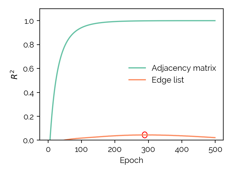
The previous post from April this year can be found here. In that post I described the general idea of reverse-engineering QUBO matrices and showed some preliminary results. The gist of that is as follows: Classification works really well, i.e. at that point classifying between 11 problems showed very high accuracy above 99.8%, while reverse-engineering (the following regression task: QUBO -> original problem, e.g. the TSP graph underlying a given TSP QUBO) is a bit more split. In the following table it can be seen that mostly graph-based problems are easily reverse-engineered (the +), while others such as Set Packing or Quadratic Knapsack cannot be fully reverse-engineered. Note that this table is directly from the Github project.

Problem	Reversibility	Comment
Graph Coloring	+	Adjacency matrix found in QUBO.
Maximum 2-SAT	?	Very complex to learn, but possible? C.f. `m2sat_to_bip.py` in `contrib`.
Maximum 3-SAT	?	Very complex to learn, but possible?
Maximum Cut	+	Adjacency matrix found in QUBO.
Minimum Vertex Cover	+	Adjacency matrix found in QUBO.
Number Partitioning	+	Easy, create equation system from the upper triangular part of the matrix (triu).
Quadratic Assignment	+	Over-determined linear system of equations -> solvable. P does not act as salt. A bit complex to learn.
Quadratic Knapsack	-	Budgets can be deduced easily (Find argmin in first row. This column contains all the budgets.). P acts as a salt -> thus not reversible.
Set Packing	-	Multiple problem instances lead to the same QUBO.
Set Partitioning	-	Multiple problem instances lead to the same QUBO.
Traveling Salesman	+	Find a quadrant with non-zero entries (w/ an identical diagonal), transpose, the entries are the distance matrix. Norm result to between 0 and 1.
Graph Isomorphism	+	Adjacency matrix found in QUBO.
Sub-Graph Isomorphism	+	Adjacency matrix found in QUBO.
Maximum Clique	+	Adjacency matrix found in QUBO.

It should be noted though that there is still some variance in the data (judging by the $R^2$ values being far above $0$ ) that can be explained by the models I trained. Thus, while the table says that 5 problems are not reversible, for example $20\%$ of the data is still reversed by the model, which is not bad. The details of the exact reversibility will either be published in a paper or are available by contacting me, since this is too much for this blog post. This also includes 3 more problem types (Graph Isomorphism, Sub-Graph Isomorphism and Maximum Clique), bringing the total to 14 supported problem types. 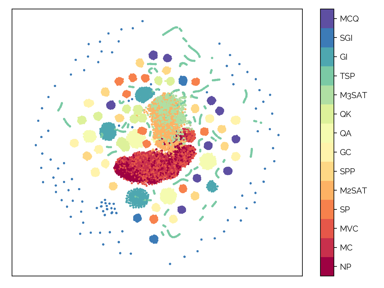The very nice t-SNE plot for the classification is seen next.

Due to supporting the translation of 14 problem types into QUBOs, I've decided to publish the project as a package on pypi. There are likely more problem types coming up that will be supported as well, thus this package may become useful for others in the industry. The exact list of problems implemented is:

Number Partitioning (NP)
Maximum Cut (MC)
Minimum Vertex Cover (MVC)
Set Packing (SP)
Maximum 2-SAT (M2SAT)
Set Partitioning (SP)
Graph Coloring (GC)
Quadratic Assignment (QA)
Quadratic Knapsack (QK)
Maximum 3-SAT (M3SAT)
Traveling Salesman (TSP)
Graph Isomorphism (GI)
Sub-Graph Isomorphism (SGI)
Maximum Clique (MCQ)

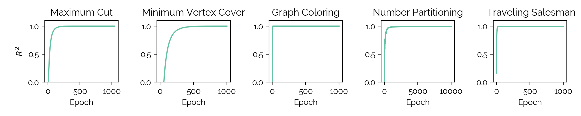
Now, a few more things were investigated: First of all, the classification and reverse-engineering was extended to a more generalized dataset which does not contain just one problem size (and thus one QUBO size), but multiple, which are then zero-padded. So for instance, a dataset consisting of $64\times64$ QUBO matrices could also contain zero-padded QUBOs of size $32\times32$ or $16\times16$ . This worked really well, though some problem types (mostly the ones that scale in $n^2\times{}n^2$ ) required more nodes in the neural network to reach the same $R^2$ and thus the same model performance, since the model had to differentiate between the different problem sizes in the dataset.

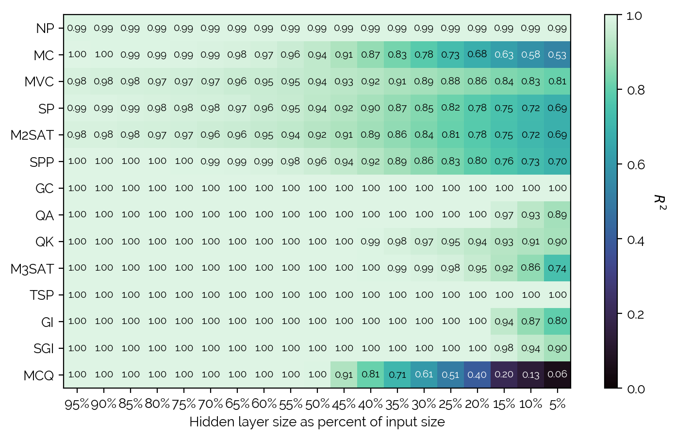
Further, the general redundancy in QUBOs was studied: AutoEncoders were trained for each problem with differing hidden layer sizes, and the resulting $R^2$ when reconstructing the input QUBO was saved. A summary of the data is seen in the figure below.

Doing a step-back, it can be seen that there is in general a lot of redundancy. There are also some interesting differences between the problem types in terms of how much redundancy there is - for instance, TSP or GC have so much redundancy that even a hidden layer size of 204 (from the input size of 4096) is enough to completely reconstruct the QUBO. Mostly the QUBOs that scale in $n^2\times{}n^2$ and QUBOs that in general have a very lossy translation. It is surprising that graph-based problems that have an adjacency matrix do not allow much compression and thus do not have as much redundancy (cf. Maximum Cut or Minimum Vertex Cover).

The project also includes a lot of attempts at breaking classification. The goal here is to find a different representation of the QUBOs that is extremely similar (so all the QUBOs are similar) while making sure they still encode the underlying problem and represent valid QUBOs. For this, the following AutoEncoder architecture (shown for 3 problem types, but easily extendable to more) was used.

It includes reconstruction losses, a similarity loss (just MSE) between the hidden representations and a qbsolv loss (not shown) that ensures that the hidden representations are valid QUBOs (which otherwise would not be the case, and which makes this whole exercise void). The qbsolv loss is based on a special layer as proposed in Vlastelica et al., and the exact implementation in QUBO-NN can be found here.

This wraps up this post for now - of course there is still a lot more to discuss, but this is for another post. Check out the Github repository if you are interested.

References:

Vlastelica et al., "Differentiation of Blackbox Combinatorial Solvers"

Published on 2021-07-12

# The Case for Alphalerts

Alphalerts is the latest business attempt of mine. Why another financial alerting service though?

Current services that allow some sort of alerting are very restricted. The reason is simple - they offer alerting as some sort of by-thought of their main product, be it brokerage services or buy/sell alerts. Note: Buy/sell alerts are different from 'general' alerts. The former often rather seems like a glorified roboadvisor. Ideas here are sentiment analysis or unusual options activity (but there are a lot more..). This business tries to actively make this its core offering: Alerting of any kind of financial event there can be.

You want to get alerted when Tech companies with high Q/Q earnings growth drop? You want to get alerted when Cryptocurrencies start to pump (and dump)? You're a CEO that just wants to buy your favorite stock at a favorable price, but don't want a standing limit order? Create a simple alert on Alphalerts that sends you an SMS or App alert when that happens.

The platform makes querying the database easy, and adds elements that explain the KPIs to people who know less while making sure power users have a lot of options.

See the Figure below for an example. The query looks for Tech companies with high Q/Q earnings growth (over 100%), with a market capitalization between 50M and 1B and a drop of over 4%.

Of course, the product is still far from being completely done. But the core functionality is there. There are also special KPIs that are supported: For instance, one can also get alerted when the live Equity Put/Call Ratio crosses a threshold. More are planned for the future. The current financial vehicles supported are US stock options, NYSE and Nasdaq stocks and cryptocurrencies. There is also a large (but still incomplete) knowledge base and good documentation, which makes it easy for professionals to understand what exactly is being offered, while giving newbies the opportunity to learn and become pro, since the KPIs that are offered are pure financial knowledge (things like institutional ownership, earnings growth, dividends.. and so on). Lastly, of course there is an App which can be used to manage queries on the go, but also receives notifications (i.e. the alerts themselves), if one likes.

I think in general, this is a very nice tool with a laser focus on financial alerting.

Published on 2021-07-10

# List of QUBO formulations

Below a list of 112 optimization problems and a reference to the QUBO formulation of each problem is shown. While a lot of these problems are classical optimization problems from mathematics (also mostly NP-hard problems), there are interestingly already formulations for Machine Learning, such as the L1 norm or linear regression. Graph based optimization problems often encode the graph structure (adjacency matrix) in the QUBO, while others, such as Number Partitioning or Quadratic Assignment encode the problem matrices s.t. a non-linear system of equations can be found in the QUBO. The quadratic unconstrained binary optimization (QUBO) problem itself is a NP-hard optimization problem that is solved by finding the ground state of the corresponding Hamiltonian on a Quantum Annealer. The ground state is found by adiabatically evolving from an initial Hamiltonian with a well-known ground state to the problem Hamiltonian.

This is by no means the definite list of all QUBO formulations out there. This list will grow over time.

For 20 of these problems the QUBO formulation is implemented using Python (including unittests) in the QUBO-NN project. The Github can be found here.

Problem	QUBO formulation
Number Partitioning (NP)	Glover et al.²
Maximum Cut (MC)	Glover et al.²
Minimum Vertex Cover (MVC)	Glover et al.²
Set Packing (SP)	Glover et al.²
Set Partitioning (SPP)	Glover et al.²
Maximum 2-SAT (M2SAT)	Glover et al.²
Maximum 3-SAT (M3SAT)	Dinneen et al.⁹
Graph Coloring (GC)	Glover et al.²
General 0/1 Programming (G01P)	Glover et al.²
Quadratic Assignment (QA)	Glover et al.²
Quadratic Knapsack (QK)	Glover et al.²
Graph Partitioning	Lucas⁷
Decisional Clique Problem	Lucas⁷
Maximum Clique Problem	Chapuis¹⁹
Binary Integer Linear Programming	Lucas⁷
Exact Cover	Lucas⁷
3SAT	Lucas⁷
Maximal Independent Set	Djidjev et al.⁸
Minimal Maximal Matching	Lucas⁷
Set Cover	Lucas⁷
Knapsack with Integer Weights	Lucas⁷
Clique Cover	Lucas⁷
Job Sequencing Problem	Lucas⁷
Hamiltonian Cycles Problem	Lucas⁷
Minimal Spanning Tree	Lucas⁷
Steiner Trees	Lucas⁷
Directed Feedback Vertex Set	Lucas⁷
Undirected Feedback Vertex Set	Lucas⁷
Feedback Edge Set	Lucas⁷
Traveling Salesman (TSP)	Lucas⁷
Traveling Salesman with Time Windows (TSPTW)	Papalitsas et al.¹, Salehi et al.⁶⁷
Graph Isomorphism	Calude et al.⁴
Subgraph Isomorphism	Calude et al.⁴
Induced Subgraph	Calude et al.⁴
Capacitated Vehicle Routing (CVRP)	Irie et al.⁵, Feld et al.³¹
Multi-Depot Capacitated Vehicle Routing (MDCVRP)	Harikrishnakumar et al.⁶
L1 norm	Yokota et al.³
k-Medoids	Bauckhage1 et al.¹⁰
Contact Map Overlap Problem	Oliveira et al.¹¹
Minimum Multicut Problem	Cruz-Santos et al.¹²
Broadcast Time Problem	Calude et al.¹³
Maximum Common Subgraph Isomorphism	Huang et al.¹⁴
Densest k-subgraph	Calude et al.¹⁵
Longest Path Problem	McCollum et al.¹⁶
Airport Gateway Assignment	Stollenwerk et al.¹⁸
Linear regression	Date et al.¹⁷
Support Vector Machine	Date et al.¹⁷
k-means clustering	Date et al.¹⁷
Eigencentrality	Prosper et al.²⁰
Container Assignment Problem	Phillipson et al.²¹
k-colorable subgraph problem	Rodolfo et al.²²
Routing and Wavelength Assignment with Protection	Oylum et al.²³
Aircraft Loading Optimization	Giovanni et al.²⁴
Linear least squares / system of linear equations	Ajinkya et al.²⁵
Traffic Flow Optimization	Neukart et al.²⁶
Permutation Synchronization	Tolga et al.²⁷
Max-Flow Problem	Krauss et al.²⁸
Network Shortest Path Problem	Krauss et al.²⁹
Structural Isomer Search Problem	Terry et al.³⁰
k-densest Common Sub-Graph Isomorphism	Huang et al.³²
Community Detection	Negre et al.³³
Nurse Scheduling problem	Ikeda et al.³⁴
Aircraft Loading Optimization	Pilon et al.³⁵
PageRank	Garnerone et al.³⁶
Ramsey numbers	Gaitan et al.³⁷
Generalized Ramsey numbers	Ranjbar et al.³⁸
Transaction Settlement	Braine et al.³⁹
Sensor placement problem in water distribution networks	Speziali et al.⁴⁰
Fault Detection and Diagnosis of Graph-Based Systems	Perdomo-Ortiz et al.⁴¹
Bounded-Depth Steiner Trees	Liu et al.⁴²
Graph Matching with Permutation Matrix Constraints	Benkner et al.⁴³
Gaussian Process Variance Reduction	Bottarelli et al.⁴⁴
Quantum Permutation Synchronization	Birdal et al.⁴⁵
Unit Commitment Problem	Ajagekar et al.⁴⁶
Heat Exchanger Network Synthesis	Ajagekar et al.⁴⁶
Garden Optimization Problem	Calaza et al.⁴⁷
Two-Dimensional Cutting Stock Problem	Arai et al.⁴⁸
Labelled Maximum Weighted Common Subgraph	Hernandez et al.⁴⁹
Maximum Weighted Co-k-plex	Hernandez et al.⁴⁹
Molecular Similarity based on Graphs	Hernandez et al.⁴⁹ (*)
Portfolio Optimization (Modern Portfolio Theory)	Palmer et al.⁵¹, Phillipson et al.⁵²
Weighted Maximum Cut	Pelofske et al.⁵³
Weighted Maximum Clique	Pelofske et al.⁵³
Satellite Scheduling	Stollenwerk et al.⁵⁴
Refinery Scheduling	Ossorio-Castillo et al. ⁵⁵
Job Shop Scheduling	Venturelli et al.⁵⁶
Extended Job Shop Scheduling with Autonomous Ground Vehicles	Geitz et al.⁷³
Parallel Flexible Job Shop Scheduling	Denkena et al.⁵⁷
Bin Packing with Integer Weights	Lodewijks⁵⁸ (alternative: ref)
Number Partitioning with m sets	Lodewijks⁵⁸
Graph Partitioning with m sets	Lodewijks⁵⁸
Subset Sum Problem	Lodewijks⁵⁸
Numerical Three-Dimensional Matching	Lodewijks⁵⁸
Social Workers Problem	Adelomou et al.⁵⁹
EV-Bus Charging Scheduling Problem	Yu et al.⁶¹
Vehicle Routing Problem	Borowski et al.⁶⁰
Robot Path Planning	Finžgar et al.⁶²
Scheduling on Undirected Hamiltonian Paths	Rieffel et al.⁶³
Market Graph Clustering	Hong et al.⁶⁴
Balanced k-Means Clustering	Arthur et al.⁶⁵
Distance-based Clustering in general	Matsumoto et al.⁶⁶
Credit Scoring and Classification	Milne et al.⁶⁸
Dynamic Portfolio Optimization	Mugel et al.⁶⁹
Railway Dispatching and Conflict Management Optimization	Domino et al.⁷⁰
Workflow Application Scheduling	Tomasiewicz et al.⁷¹
Mirrored Double Round-robin Tournament	Kuramata et al.⁷²
Transaction Scheduling	Bittner et al.⁷⁴
Transformation Estimation	Golyanik et al.⁷⁵
Point Set Registration	Golyanik et al.⁷⁵
Maximum Cardinality Matching	Vert et al.⁷⁶
Multi-car Paint Shop Optimization	Yarkoni et al.⁷⁷
Binary Paint Shop Problem	Streif et al.⁷⁸

(*) applied to Covid-19 by Jimenez-Guardeño et al.⁵⁰

Note that a few of these references define Ising formulations and not QUBO formulations. However, these two formulations are very close to each other. As a matter of fact, converting from Ising to QUBO is as easy as setting $S_{i} \rightarrow 2x_i - 1$ , where $S_i$ is an Ising spin variable and $x_i$ is a QUBO variable.

Published on 2021-06-10

# Quantum Annealing Hamiltonian Example Calculation

Let's calculate quickly what happens.

We have an extremely simple Number Partitioning problem consisting of the set of numbers $\{1, 2, 3\}$ . It has an optimal solution, which is splitting the set into two subsets $\{1, 2\}$ and $\{3\}$ .

The Ising formulation for Number Partitioning is given as $A(\sum_{j=1}^{m}n_{j}x_{j})^2$ , where $n_j$ is the j-th number in the set. Thus, with $A=1$ , for the given set the result is $(x_1 + 2x_2 + 3x_3)^2 = x_1x_1 + 4x_1x_2 + 6x_1x_3 + 4x_2x_2 + 12x_2x_3 + 9x_3x_3$ . Now, the Hamiltonian for an Ising formulation is very simple: Replace $x_i$ by a Pauli Z Gate. We can now write the Hamiltonian using QuBits (with an exemplary QuBit state):

\langle{}010|Z_1Z_2Z_3|010\rangle{}

Thus, we can evaluate the cost of a possible set of subsets by using QuBits. For instance, a state $|010\rangle{}$ means that the numbers 1 and 3 are in one subset and the number 2 is in another subset. It should be noted that $\langle{}1|Z_i|1\rangle{} = -1$ and $\langle{}0|Z_i|0\rangle{} = 1$ .

More specifically (where $x_i = Z_i$ ), the Quantum formulation for our problem is:

\langle{}010|x_1x_1 + 4x_1x_2 + 6x_1x_3 + 4x_2x_2 + 12x_2x_3 + 9x_3x_3|010\rangle{}

Here, we have $\langle{}0|x_1|0\rangle{} = 1$ , $\langle{}1|x_2|1\rangle{} = -1$ and $\langle{}0|x_3|0\rangle{} = 1$ . Thus, the total cost is:

$\langle{}010|x_1x_1 + 4x_1x_2 + 6x_1x_3 + 4x_2x_2 + 12x_2x_3 + 9x_3x_3|010\rangle{} = 1 - 4 + 6 + 4 - 12 + 9 = 4$ .

Note that one of the the optimal solutions is:

$\langle{}001|x_1x_1 + 4x_1x_2 + 6x_1x_3 + 4x_2x_2 + 12x_2x_3 + 9x_3x_3|001\rangle{} = 1 + 4 - 6 + 4 - 12 + 9 = 0$ .

Another one would have been the state $|110\rangle{}$ .

In summary, we can now adapt a bunch of QuBits to evaluate the goodness of a solution. This in turn opens interesting possibilities..

References:

Lucas, Andrew. "Ising formulations of many NP problems.", 2014

Published on 2021-05-14

# A note on Adiabatic Evolution in Quantum Annealing

In a lot of introductory literature about Quantum Annealing, Adiabatic Quantum Computing (AQC) and Quantum Annealing (QA) are explained very well, but one crucial connection seem to always be amiss.. What exactly is evolution, or adiabatic evolution?

First, the Hamiltonian of a system gives us the total energy of that system. It basically explains the whole system (what kind of kinetic or potential energy exists, etc). The ground state of a given Hamiltonian is the state associated with the lowest possible total energy in the system. Note that finding the ground state of a system is extremely tough. A problem such as the Traveling Salesman Problem (TSP) is then converted into a formulation (QUBO or Ising) for which a Hamiltonian is set up easily.

Quantum Annealing works as per AQC as follows:

Set up the problem Hamiltonian for our problem, s.t. the ground state of the Hamiltonian corresponds to the solution of our problem.
Set up an initial Hamiltonian for which the ground state is easily known and make sure the system is in the ground state.
Adiabatically evolve the Hamiltonian to the problem Hamiltonian.

Adiabatic evolution follows the adiabatic theorem in that the evolution should not be too fast, else the system could jump into the next excited state above the ground state, which would result in a sub-optimal solution in the end. The general formula is as follows:

$\mathcal{H}_t = s(t) \mathcal{H}_i + (1 - s(t)) \mathcal{H}_f$ ,

where $\mathcal{H}_i$ is the initial Hamiltonian and $\mathcal{H}_f$ is the problem Hamiltonian. The paramater $s(t)$ is modified over time. In the beginning, the system (or time-dependent) Hamiltonian consists solely of the initial Hamiltonian. In the end, it consists solely of the problem Hamiltonian (and is hopefully still in the ground state, if the adiabatic theorem was followed).

Setting up Hamiltonians consists of translating the TSP instance to an Ising spin glass problem instance. The Hamiltonian of that problem is very well known, and by translating to an Ising problem, one automatically encodes the problem in a way s.t. minimizing the Hamiltonian (i.e. minimizing the total energy and thus getting into the ground state) automatically minimizes the Ising spin glass instance and thus the TSP instance.

With the Hamiltonians out of the way, a huge question marks sits with the adiabatic evolution part. What is going on here? The figure below shall help build an intuition.

One can see different system Hamiltonians over time and the corresponding ground state (black dot) of all possible states. The experiment would now start with the light blue Hamiltonian and over time slowly change to the problem Hamiltonian (dark purple). Thus, we are modifying the energy landscape over time! Looking back at the time-dependent Hamiltonian equation further above, this suddenly makes sense. The time-dependent Hamiltonian changes over time in that it consists of both the initial Hamiltonian and problem Hamiltonian with different fractions. Thus, the energy landscape changes over time in that it first consists solely of the initial Hamiltonian and later more and more of the problem Hamiltonian. So the literature is not missing a description of adiabatic evolution after all. Hopefully though, this visualization helps people out there understand easier the intuition behind it.

There are quite a few more topics to cover, but this post ends here to keep things short and concise. More will likely follow.

A project this was related to is QUBO-NN.

References:

McGeoch, Catherine C. "Adiabatic quantum computation and quantum annealing: Theory and practice."
Lucas, Andrew. "Ising formulations of many NP problems.", 2014

Published on 2021-05-14

# Multiplying large numbers with Neural Networks

When working on QUBO-NN, one of the problem types (specifically: Quadratic Knapsack) was causing issues in that a good neural network (with a decent $R^2$ coefficient) could not be trained. One of my ideas was that a possible cause could be the large numbers that had to be multiplied to get to a solution. Judging from this stackexchange post, I was kind of right. In the end, it was not the main cause, but it did influence the number of nodes in the neural network needed to train decent models.

I decided to do a small experiment to test this out.

First, and this is also known in the literature (though the publication is rather old), it gets tougher to train a neural network to multiply numbers, the larger they become. The first experiment is set up as follows. The dataset consists of 10000 randomly generated numbers in the range 1 to n, where n is varied across configurations (50, 200, 500, 2000). The neural network architecture consists of just one hidden layer of size 20 (and this is fixed). The optimizer of choice is Adam with a learning rate of 0.005, and the activation function is ReLU. I always train for 500 epochs and use a batch size of 10. The dataset is normalized between 0 and 1.

The next figure shows an interesting result.

In the first 300 epochs, one would assume that the model for n=2000 is a failure with a $R^2$ coefficient below 0.96. The jumps are also extremely interesting --- each model has its own jump in the $R^2$ coefficient, and the lower n, the earlier the jump happens.

Future work would include training for thousands of epochs and observing whether the worst model (with n=2000) still improves further.

A next experiment shows that including more nodes helps immensely (c.f. the next figure). The worst model (n=2000) is trained on a neural network with hidden layer size 100 (instead of 20).

The solution proposed in the previously linked stackexchange post to use the logarithm works extremely well: For the worst model (with n=2000), after just 6 epochs the $R^2$ coefficient is at $0.9999999999987522$ . Damn. The same previously cited publication supports this idea of using the logarithm with similar results. The idea is simple: Before training, transform the input and target using the natural logarithm. Afterwards, if one requires the actual numbers, simply take the exponential of the result.

In summary, training neural networks to multipy large numbers quickly leads to huge training times (with a large number of epochs required to reach a good $R^2$ coefficient). The logarithm trick helps, since addition is trivial for a neural network to learn. Adding more nodes also helps.

The source code for the experiments can be found here.

Published on 2021-05-10

# QUBO NN - Reverse Engineering QUBO matrices

I've been trying to create a reverse-engineering pipeline for QUBO matrices, and it has been quite interesting.. Not as easy as one would think. So the story here is quite simple: Since the current global Quantum Compute is concentrated across a few companies and institutions, what if these institutions read your QUBO matrices and infer secret information. For instance, say you're a hedge fund that quantifies some secret alpha - they trust you not to steal that and thereby instantly devalue their alpha.

In classical compute (with cloud computing) there are interesting ideas such as homomorphic computation (using homomorphic encryption). The goal of the project is to create a pipeline that can classify the problem a given QUBO matrices is based on and then infer the parameters that the QUBO matrix has been generated with. Below a schematic overview is given.

I used neural networks for both steps. We do neural network multi-classification (step a) and neural network regression (step b). Now, the results are quite promising.

The first step, i.e. classifying, is pretty straightforward. I set up 11 problems and generated 100000 problem instances each. The chart below shows how after just 40 epochs we are already near 0 in terms of error rate:

The second step is not as straightforward. 5 of the problems turned out to be trivially reversible. The $R^2$ coefficient comes very close to 1.0:

Maximum Cut needs additional thoughts (the blog post about that can be found here) - specifically, the output needs to be an adjacency matrix and not an edge list. This is actually very important:

As for the rest, I am actively looking into it. A table with all 11 problems and their reversibility can be found here. Some problems such as Quadratic Assignment (QA) I assumed to be non-reversible, but I was wrong. The QUBO of a QA problem defines an over-determined linear system of equations, which can be solved by a neural network. However, the best I got so far is a $R^2$ coefficient of 99%. Not bad, but could be better. The problem I really struggled with so far is Maximum 2-SAT. I am not 100% sure yet, but my hunch is that it is simply too complex for a standard fully connected neural network.

For anyone interested, the Github repository can be found here.

An update post can be found here.

Published on 2021-04-04

# Learning with Errors Problem Example in Post Quantum Cryptography

There are a multitude of approaches in post-quantum cryptography that promise security in a world where Quantum Computers are powerful enough to break RSA using Shor's algorithm. Some interesting ones include isogeny based ones or lattices, to which Learning with Errors (LWE) belongs. The contribution of this post is a simple and easily modifiable example on how asymmetric encryption based on LWE works.

Initially, B creates an over-defined and solvable system of equations such as:

5a + 4b + c = 17 mod 20
3a + 10b + c = 19 mod 20
10a + 5b + 3c = 14 mod 20

with a=2, b=1 and c=3. Those three numbers are the private key of B.

Next, B adds errors to the equation system:

5a + 4b + c = 17+1 mod 20
3a + 10b + c = 19-2 mod 20
10a + 5b + 3c = 14+1 mod 20

and denotes the coefficients and the wrong values the public key:

5   4   1   18
3   10  1   17
10  5   3   15

with modulo 20.

A now wants to encrypt a message using B's public key and send it to B. She goes bit by bit. We start with the very first bit of the message, which is for example 1. For each row of the public key she flips a coin. She sums up the rows come up with tails. Let's for example assume row 1 and 3 came up. She sums up the coefficients and values and ends up with:

15a + 9b + 4c = 18+15 mod 20 = 13 mod 20

Depending on the message bit, which in our example is 1, she adds an error:

a large one if the bit is 1
a small one if the bit is 0

In our case we change 13 mod 20 to for example 2 mod 20. A sends to Bob the coefficients and the wrong value:

15  9   4   2

B now inserts the private key and calculates:

15a + 9b + 4c = 15*2 + 9*1 + 4*3 = 51 mod 20 = 11 mod 20

Since the value transmitted by A is 2 and this is a large error, B assumes the bit was 1. Likewise, if the bit would have been 0, A would have for example sent 12 mod 20 instead of 2 mod 20.

The reason this scheme works is that it is very easy to add errors to the system of equations, but very tough to find the errors when a, b, c are unknown.

And where is the lattice in this? The public key of B can be seen as a set of basis vectors in a lattice and the attacker needs to solve the Closest Vector Problem to find the good (real) vectors, which is very tough (polynomial runtime algorithms approximate the solution only within exponential quality).

Published on 2021-03-21

# I accidentally tried to train 1 Quadrillion parameters (and a story of structural bias)

What a rookie mistake, but a funny one indeed. So it all started with me seeing what I'd mistakenly called avoidable bias.

The train error rate bottoms out at roughly 28, which is NOT ~0 and definitely not satisfying. This looks like underfitting and a big chunk of avoidable bias, at first. As per theory, one should increase the number of parameters to deal with underfitting, so that's exactly what I did. One thing to keep in mind - statistical error (or variance), i.e. the difference between train and test errors increase proportionally with the number of parameters. So if we overshoot, we overfit badly. In that case, increasing the number of data points might help.

With all this in mind, I just went ahead. Now, what I kind of forgot is how quickly the number of parameters grow in fully connected networks. The issue with the data is that it is very high dimensional - the input size is 4096 and the output size was 180 at this stage. With literally zero hidden layers and just that input and output, we already have 4096 * 180 = 737280 parameters. So anyways, I started with a hidden layer of 2000, 5000, 10000 and at some point ended up with two massive 50000 node layers. Also tested 10 $\times{}$ 10000 layers at some point too. Let's do some quick maths:

4096 * 50000 ** 2 * 180 = 1.8432e+15

That's ~1.8 Quadrillion parameters. I was astonished as to why the so called 'avoidable' bias was not going away. And of course, training the models became very slow too. Further, the bias stayed at an even higher level with a higher number of parameters!

Two main takeaways here:

This was structural bias (unavoidable)
Training 1.8 Quadrillion parameters lead to the bias staying elevated since training is too inhibited. After the same amount of time (when compared to the simple 700k parameter model) we simple haven't learnt anything and thus the train error stays high.

After changing my data I ended up with no structural bias and a bit of avoidable bias. I upped the number of training epochs and got to close to 0 error loss.

Observe below the relationships between different types of errors and model complexity (number of parameters) or number of training epochs.

The data was related to this post and this project. Specifically, I tried to predict the parameters (i.e. the exact graph) that lead to a 64 $\times{}$ 64 QUBO matrix of a Maximum Cut problem. At first, I encoded the output as the list of edge tuples (since we had 90 edges pre-defined, that's 180 nodes). I am not 100% sure where the structural bias is coming from, but my hunch is that it is the ordering of edges. Now, it's not as simple as saying that the edges are stored in a dict and thus they're ordered in a random way - that's not the case since Python 3.7. The edges (=dict) keep insertion order. But what if the insertion itself was random? That is exactly the case here - I am using gnm_random_graph which generates edges randomly in random order and inserts them randomly. And randomness is structural bias that cannot be learnt by a neural network. So there you have it. I ended up predicting a full adjacency matrix, which gets rid of the structural bias. Works now, nice!

Published on 2021-03-16

# Oblivious Transfer Example With Physically Unclonable Function (PUF)

Physically Unclonable Functions (PUFs) are an extremely interesting and hot topic in cryptography. The basic gist is, you have a certain physical object that cannot be cloned due to the extremely intricate properties of it (e.g. the atomic structure of a DVD) that depend on the manufacturing process. The assumption is that each DVD is unique when looking at its atomic structure. Now, when measuring the reflection of a DVD with a high precision device of some sort, these differences show up. Imagine you put a chip in a capsule which inner walls consist of such reflective material. The chip has a device that measures the reflection and based on that generates a key pair (a public and a private one). This public key pair can be used to communicate with the device and identify it, and if someone were to try to tamper with the device by drilling into it - the reflective material would break, changing the measurement and thus the public key. Lastly, an additional digital signature on the device ensures that anyone can check for tampering (the public key is contained in the digital signature). The most important part is that the device is secret-free. The 'secret' is the material and there is no way to clone that material to re-use the secret and there is no way to find out the private key without breaking the whole thing. Pretty cool concept.

PUFs can be used for many cryptographic primitives, one of which is Oblivious Transfer (OT). The point of OT is: A wants to get a certain information from B based on A's choice. B should stay oblivious of the choice of A in the process however, and A should not be able to get all of the options from B. Pretty specific, I know. But being a cryptographic primitive has lots of uses. See the paper Founding Cryptography on Oblivious Transfer - Efficiently, which builds secure two-party computation based on OT.

Anyways, enough of introduction. The main contribution of this small post is to show an example calculation of how Oblivious Transfer would work with PUFs. In the figure below you can see how the scheme works. A uses the PUF to create a list of challenge-response pairs (CRPs) and sends over the PUF to B. B chooses two values x0 and x1 and sends those to A. A now chooses one of those and sends back the challenge XOR'd with the chosen value. B measures the response of the PUF of the two challenges v XOR x0 and v XOR x1. The interesting thing here is that depending on the choice of A, one of those challenges ends up being the real challenge C of A (e.g. if A chooses x0, v XOR x0 = C XOR x0 XOR x0 = C). B sends both choices (s0, s1) back, but XOR'd with both responses. A chooses the correct one based on its choice and since it has the response for C, can compute y0 XOR R = s0 (if continuing with the example of choosing x0).

Now, an example calculation.

s0 = 5
s1 = 6

# A chooses random C and a choice b (can be 0 or 1).
C = 5412
R = 7777
b = 1

# B chooses random x0, x1.
x0 = 44
x1 = 66

# A calculates (remember, A chose 1):
v = C ^ x1 = 5412 ^ 66 = 5478

# B measures the two challenges.
R0 = v ^ x0 = 5478 ^ 44 = 5450 = 9999
R1 = v ^ x1 = 5478 ^ 66 = 5412 = 7777

# B sends back both choices XOR'd with both responses.
y0 = s0 ^ R0
y1 = s1 ^ R1

# A XORs the second reply from B (first one is garbage) and gets the choice value they wanted.
s1 = y1 ^ R = 6

In summary, what we just observed: A lets B compute both options so B doesn't know the chosen bit b. And B computes both options in a way that the option not chosen is garbled, while the option chosen can be deduced by A.

Published on 2021-03-13

# QUBOs for TSP and Maximum-3SAT

Generating QUBOs for Maximum 3-SAT and the Traveling Salesman Problem (TSP) was a bit tougher than the other 9 problems that were outlined in https://arxiv.org/pdf/1811.11538.pdf. In this post I would like to give a quick example on how one would do so. For reference, the context of this is this project. To understand this post, it is required to read the arxiv paper above. Else I believe the code won't make any sense.

For Maximum 3-SAT, the following clauses are given:

(x_1 \lor x_2 \lor x_3), (\overline{x_1} \lor x_2 \lor x_3), (x_1 \lor \overline{x_2} \lor x_3), (\overline{x_1} \lor x_2 \lor \overline{x_3})

In code (c.f. here) it looks like this, where the number is the variable index and the boolean denotes the state of the variable:

problem = Max3SAT(
    [
        ((0, True), (1, True), (2, True)),
        ((0, False), (1, True), (2, True)),
        ((0, True), (1, False), (2, True)),
        ((0, False), (1, True), (2, False))
    ],
    3
)

The QUBO matrix we are looking for looks like this:

[
    [0.0, -1.0, 1.5, -0.5, 0.5, -0.5, 0.5],
    [-1.0, 1.0, 0.0, -0.5, -0.5, 0.5, -0.5],
    [1.5, 0.0, -1.0, -0.5, -0.5, -0.5, 0.5],
    [-0.5, -0.5, -0.5, 2.0, 0.0, 0.0, 0.0],
    [0.5, -0.5, -0.5, 0.0, 1.0, 0.0, 0.0],
    [-0.5, 0.5, -0.5, 0.0, 0.0, 1.0, 0.0],
    [0.5, -0.5, 0.5, 0.0, 0.0, 0.0, 0.0]
]

And as a normalized heatmap:

For Maximum 2-SAT, the QUBO formulation is really space-efficient (which is important for current architectures) and only scales with the number of variables (see arxiv link above). Awesome! For Maximum 3-SAT unfortunately we scale with both the number of variables and the number of clauses.

The code to generate a QUBO for Maximum 3-SAT is seen below. The main loop is split in two parts, one that generates the blue part of the formula below and one that generates the green part. To be specific, the formula is just for 3 variables, so it's not general. The green part is simply the combinations of all variables (e.g. if you have 5 variables, there's 10 combinations).

\sum^{m}_{i=1} \textcolor{blue}{((1 + w_i)(y_{i1}+y_{i2}+y_{i3})} - \textcolor{green}{y_{i1}y_{i2} - y_{i1}y_{i3} - y_{i2}y_{i3} - 2w_i}

Here's the code:

def gen_qubo_matrix(self):
    n = self.n_vars + len(self.clauses)
    Q = np.zeros((n, n))

    # Clauses is a list of 3-tuples of 2-tuples.
    # Eg: [((0, True), (2, True), (3, False)), ((1, True), (3, False), (4, True))]
    # So we loop through all tuples and find the type of it.
    # There are 4 types: (True, True), (True, False), etc.
    for i, clause in enumerate(self.clauses):
        clause_idx = self.n_vars + i
        Q[clause_idx][clause_idx] += 2

        # (1 + w1) * (x1 + x2 + x3) = x1 + x2 + x3 + w1x1 + w1x2 + w1x3
        # (1 + w1) * ((1 - x1) + x2 + x3) = -x1 + x2 + x3 + w1 -w1x1 +w1x2 +w1x3
        # (1 + w1) * ((1 - x1) + x2 + (1 - x3)) = -x1 + x2 -x3 + 2w1 -w1x1 +w1x2 -w1x3
        for item in clause:
            item_idx = item[0]
            val = item[1]
            if val:
                Q[item_idx][item_idx] -= 1
                Q[clause_idx][item_idx] -= .5
                Q[item_idx][clause_idx] -= .5
            if not val:
                Q[item_idx][item_idx] += 1
                Q[clause_idx][clause_idx] -= 1
                Q[clause_idx][item_idx] += .5
                Q[item_idx][clause_idx] += .5

        # -x1x2 -x1x3 -x2x3
        # -(1-x1)x2 -x1x3 -x2x3 = -1 +x1x2
        # -(1-x1)(1-x2) -x1x3 -x2x3 = -1 -2x1x2 +x1 +x2
        for (item1, item2) in itertools.combinations(clause, 2):
            idx1 = item1[0]
            idx2 = item2[0]
            val1 = item1[1]
            val2 = item2[1]
            if val1 and val2:
                Q[idx1][idx2] += .5
                Q[idx2][idx1] += .5
            if not val1 and val2:
                Q[idx2][idx2] += 1.
                Q[idx1][idx2] -= .5
                Q[idx2][idx1] -= .5
            if val1 and not val2:
                Q[idx1][idx1] += 1.
                Q[idx1][idx2] -= .5
                Q[idx2][idx1] -= .5
            if not val1 and not val2:
                Q[idx1][idx2] += 1.
                Q[idx2][idx1] += 1.
                Q[idx1][idx1] -= 1.
                Q[idx2][idx2] -= 1.

    return Q

As you can see, it's longer than most other QUBO generators in the project. The matrix that is generated also looks very intricate. A small note for newcomers to QUBOs: Whenever there is a variable that is not on the diagonal, e.g. $x_1x_2$ , one splits the constant in two. This is why you see these .5 additions and subtractions. A lone variable $x_3$ would be on the diagonal at Q[3][3] and leads to no such split. What about $2x_1x_2$ ? Well, we end up with $\pm1$ .

As for TSP, the problem is defined as a distance matrix between the nodes of the graph and a constraint c. For instance, below we see three nodes with distances normalized to the range 0 to 1.

dist_matrix = [
    [0, 1/3., 2/3.],
    [1/3., 0, 1/3.],
    [1, 1/3., 0]
]

The resulting QUBO matrix looks like this (note: the constraint is set to 400):

[
    [-800.00, 800.00, 800.00, 800.00, 0.00, 0.00, 800.00, 3.33, 10.00],
    [800.00, -800.00, 800.00, 0.00, 800.00, 0.00, 3.33, 800.00, 3.33],
    [800.00, 800.00, -800.00, 0.00, 0.00, 800.00, 6.67, 3.33, 800.00],
    [800.00, 3.33, 10.00, -800.00, 800.00, 800.00, 800.00, 0.00, 0.00],
    [3.33, 800.00, 3.33, 800.00, -800.00, 800.00, 0.00, 800.00, 0.00],
    [6.67, 3.33, 800.00, 800.00, 800.00, -800.00, 0.00, 0.00, 800.00],
    [800.00, 0.00, 0.00, 800.00, 3.33, 10.00, -800.00, 800.00, 800.00],
    [0.00, 800.00, 0.00, 3.33, 800.00, 3.33, 800.00, -800.00, 800.00],
    [0.00, 0.00, 800.00, 6.67, 3.33, 800.00, 800.00, 800.00, -800.00]
]

And as a normalized heatmap:

TSP is unfortunately rather inefficient to encode. For $n$ nodes, we have a $n * n$ distance matrix and a $n^2 * n^2$ QUBO matrix! Below is the code for generating a TSP QUBO (c.f. here for more context):

def gen_qubo_matrix(self):
    n = len(self.dist_matrix)
    Q = np.zeros((n ** 2, n ** 2))

    quadrants_y = list(range(0, n ** 2, n))
    quadrants_x = quadrants_y[1:] + [quadrants_y[0]]

    # The diagonal positive constraints
    for start_x in quadrants_y:
        for start_y in quadrants_y:
            for i in range(n):
                Q[start_x + i][start_y + i] = 2 * self.constraint

    # The distance matrices
    for (start_x, start_y) in zip(quadrants_x, quadrants_y):
        for i in range(n):
            for j in range(n):
                if i == j:
                    continue
                Q[start_x + i][start_y + j] = self.P * self.dist_matrix[j][i]
            Q[start_x + i][start_y + i] = 2 * self.constraint

    # The middle diagonal negative constraints
    for start_x in quadrants_x:
        for i in range(n):
            Q[start_x + i][start_x + i] = -2 * self.constraint
            for j in range(n):
                if i != j:
                    Q[start_x + i][start_x + j] += 2 * self.constraint

Note: P is set to 10.

This wraps up the post. I've shown an example problem instance for Maximum 3-SAT and one for TSP and code on how to generate QUBO matrices for each.

Published on 2021-02-24

# PPO - a Note on Policy Entropy in Continuous Action Spaces

I've always wondered what policy entropy really means in the context of PPO. From other posts (e.g. here by AurelianTactics - btw very cool guy saw him on the official reddit RL Discord) I know that it should continuously go down. It also corresponds to the exploration the PPO agent is taking --- high entropy means high exploration.

In this case I will be looking at continuous action spaces. Here, each action in the action space is represented by a gaussian distribution. The policy is then called a gaussian policy. In my case, I have two continuous actions (for more information, check out the post Emergent Behaviour in Multi Agent Reinforcement Learning - Independent PPO).

Now, entropy for a gaussian distribution is defined as follows: $\frac{1}{2} \log(2\pi{}e\sigma{}^2)$ . What baselines PPO does now is to simply sum the entropies across the actions axis (e.g. given a batch of 700 actions s.t. the shape is (700,2), this becomes (700,)) and then take the mean over the batch. Their inner code is equal to the definition above since $\log(a*b) = \log(a) + \log(b)$ . For reference, this is using the natural log.

This is a single entropy calculation:

tf.reduce_sum(self.logstd + .5 * np.log(2.0 * np.pi * np.e), axis=-1)

And this is taking the mean over the whole batch:

entropy = tf.reduce_mean(pd.entropy())

The right side (.5 * np.log(2.0 * np.pi * np.e)) ends up being roughly 1.41. You can now deduce, given an entropy reading, how uncertain (and thus exploratory) each action is. High entropy equals high exploration and vice versa. To quantify the above, check out the figure below:

You can see that at roughly variance = 0.242 entropy is 0.

This is how policy entropy looks for me when training two predator PPOs to catch prey:

As you can see, exploration decreases continuously. It starts with variance = 1 for both actions and ends up at variance = 0.3 after training. (starts at 2.82 = 1.41 * 2, which is incidentally the entropy for 2 actions summed up, given variance of both is 1). Nice!

Update: Some notes regarding why we take the mean.

One could argue that the logstd does not change over the 700 batch, since the policy did not change. And that is true, we actually get 700 times the same entropy number. The reason why every PPO implementation takes the mean here is two-fold.

First of all, check out the loss PPO optimizes (see paper):

L_t^{CLIP+VF+H}(\theta{}) = \mathbb{E}_t[L_t^{CLIP}(\theta{}) - c_1L_t^{VF}(\theta{}) + \textcolor{blue}{c_2H[\pi_{\theta}](s_t)}]

The blue part is the entropy, and observe how it is in the expectation $\mathbb{E}$ , for which you usually take the mean.

Secondly, autograd. One optimization idea would be to just take the first entropy number and throw away the others (so an indexing operation instead of the mean), but that would not play well with autograd, which uses the gradients to update all parameters (including the logstd parameter and thus your policy itself) in the backwards pass. Calculating the gradient of a mean is easy, but the gradient of an indexing operation? The key word here is 'differentiable indexing' and it is possible, but you only update part of your parameters (the part you indexed). In this case my hunch is that you end up only updating your policy once instead of 700 times, which defeats the purpose of a 700 batch. At that point you should just do singular updates and no batching.

Published on 2021-02-19

# Burry is sharing Heavy Metal again - his TSLA short must be bleeding

This is so hilarious I just gotta save this for the books. Michael Burry, the famous main character from The Big Short who predicted the housing market crash and made a nice 100M for himself (total net worth back then 300M), is short on TSLA. And he has started sharing heavy metal on his Twitter, which is interesting - this is portrayed in the movie as something he uses to get rid of the stress of BLEEDING CASH EVERY MONTH lol. The position must be pretty hard on his nerves. On the other hand, he just made some very good cash on his GME play.

For the record, I totally agree with him. There are quite a few indicators that the market is devolving into a bubble. Wallstreetbets for instance has gained over 6M subscribers over the GME fiasco (which I missed, but I made some money shorting it). It had 2M subscribers before, and has 8.8M now. I have personally heard of some laymen in my circle of friends that they are becoming interested in the stock market. So yea, interesting times. And then there is Bitcoin and TSLA..

So let's see how 2021 plays out. I now know that my post There is no recession coming was technically right. We basically did not have a recession in 2020, that was like a small shake-out! So maybe I will look back at this post some time in the future and agree with my past self.

While writing this post I was listening to the Heavy Metal Michael Burry shared - my god that is some good shit. I might just take a dive into that genre off of his recommendation.

Here you go: link

Update: Just found a satirical comment I posted literally at the bottom of the crash in March 2020. Everyone on WSB was balls deep in puts. Fucking hilarious.

Published on 2021-02-09

# Data Preparation is Everything - Parsing The German Commercial Register (Handelsregister)

There are three major issues with the commercial register (Handelsregister) data. First of all, every company has their own rules, e.g. in terms of appointments. Who is allowed to be appointed, when and why and with whose permission.. Thousands of combinations. Secondly, our clerks do not seem to follow the format 100%. And they make spelling mistakes sometimes. But the most glaring one is: Each register entry is ONE line of TEXT. And there is no official delimiter it seems. The clerks all kind of go with a few loose rules but yea - it is definitely not defined by a RFC or something lol. So what does this leave us with. LOTS of Regex and special rules, and it is pretty painful. But this should be known to any serious ML practitioner, that most of the work lies in data preparation.

For instance, I want you to look at this regex (which is just a small part of the data preparation pipeline):

(Die |Ist).*(ein|zwei)?.*(Gesellschaft|Vereinigung|Genossenschaft|vertritt|Vorstand|Geschäftsführer).*(ein|zwei)?.*
(vertreten|Prokuristen|vertreten.*gemeinsam|vertreten.*gemeinschaftlich|einzelvertretungsberechtigt|Vertretungsbefugnis von der Generalversammlung bestimmt)

It might not be perfect, but it gets the job done. So anyways, enough of the data preparation pipeline, how about a first result. While doing some descriptive statistics (data exploration), the first thing that interested me was the number of registrations per year over time. Check it out:

2015 we had a near recession with oil dropping and the Chinese market crashing, so it makes sense that in bad times less businesses were registered. But what is extremely surprising - in 2020 we had slightly more registrations than in 2019! What the hell? Seems like the 2020 global recession was kind of a fake recession for a certain chunk of the population.

Another thing that is interesting, but not plotted here (since it would look boring) - month over month the number of registrations are roughly the same. So there is no seasonality here. Quite interesting!

Just a note regarding the 2007 data (which is roughly 130 registrations) - the available data starts at the very end of 2007. Thus it looks like there are nearly no registrations in 2007, but in reality it's not a full year.

I will be working with this data some more and I will update this post (or create a new one). Specifically I am looking at doing Latent Semantic Analysis (LSA) and using the gensim library. Stay tuned!

Update: I have done some more analysis, specifically LSA. Note: The next few paragraphs will contain a lot of German words.

An important task is getting rid of small and common words such as 'der' (engl.: the), else one would throw off (dis)similarity measures. So for me this currently looks like that:

und oder der die das von zur nur so einer einem ein allein darum dazu für dafür
zum zu dort da grundkapital stammkapital eur dem usd gbp im mit an dem bei art
rahmen vor allem aller sowie aus in den als

These are often called 'stopwords', and we simply filter them out, which improves the LSA model considerably - we get more confident topic assignments.

Notice words like 'Stammkapital' (base capital) - they may look like they are important to the text, but if literally every text has Stammkapital included, it does not really give us any more information.

A seemingly important hyperparameter (similar to the number of clusters in clustering) is the number of topics. I am currently experimenting a bit here. Having too small of a number of topics seems to make most topics include stuff like 'Halten' (holding) which is a very important word since there are a lot of holding companies. Too many topics has duplicates as follows:

66 ['it', 'consulting', 'management', 'marketing', 'insbesondere', 'bereichen', 'it-dienstleistungen', 'gegenstand', 'vermarktung', 'zubehör']
67 ['marketing', 'insbesondere', 'dienstleistungen', 'it', 'in-', 'gegenstand', 'ausland', 'consulting', 'it-beratung', 'deren']

And then there are weird combinations such as the following. IT services and construction?!

81 ['an-', 'it-dienstleistungen', 'verbundenen', 'allen', 'trockenbau', 'alle', 'geschäften', 'nebst', 'damit', 'kauf']

Anyways, I will keep updating this post with new findings.

Published on 2021-02-07

# Hadamard Gate Transformation for 3 or more QuBits

While trying to understand Grover's Algorithm, I started wondering how exactly the Hadamard gate transformation looks like for not just one QuBit or even two, but for three or more. Ekert et al. in their paper Basic concepts in quantum computation show with Equation 12 a very nice general formula for the Hadamard gate transformation:

$H^{\bigotimes{}n}|x\rangle{} = \frac{\sum_z (-1)^{x \cdot z}|z\rangle{}}{\sqrt{2^n}}$ ,

where $\cdot$ is the element-wise product. The sum over $z$ indicates all possible states of $x$ (we're in a superposition!). For a n-length state there are $2^n$ possible states, so for 3 there are 8 states.

Assuming I'd like to apply Grover's algorithm to 3 QuBits as shown on the Qiskit page on Grover's algorithm, there is a point at which Hadamard is applied to 3 QuBits on a non-trivial state (not just $|000\rangle{}$ ). This is where the formula above comes in. Let's first calculate it through for $|000\rangle{}$ . Below I calculate the element-wise products $x \cdot z$ .

$\begin{pmatrix} 0 \\ 0 \\ 0 \end{pmatrix} \cdot \begin{pmatrix} 0 \\ 0 \\ 0 \end{pmatrix} = 0*0 + 0*0 + 0*0 = 0$

$\begin{pmatrix} 0 \\ 0 \\ 0 \end{pmatrix} \cdot \begin{pmatrix} 0 \\ 0 \\ 1 \end{pmatrix} = 0*0 + 0*0 + 0*1 = 0 \\ ...$

As you can see, they all amount to 0 here. Now, the general equation from above becomes trivial (note: $n=3$ and $x=|000\rangle{}$ ):

$H^{\bigotimes{}3}|000\rangle{} = \frac{\sum_z (-1)^0|z\rangle{}}{\sqrt{2^3}}$

$H^{\bigotimes{}3}|000\rangle{} = \frac{\sum_z 1|z\rangle{}}{\sqrt{8}}$

H^{\bigotimes{}3}|000\rangle{} = \frac{1}{\sqrt{8}} (|000\rangle{} + |001\rangle{} + |010\rangle{} + |011\rangle{} + |100\rangle{} + |101\rangle{} + |110\rangle{} + |111\rangle{})

In the last step all the sum was evaluated to its 8 possible states. This is probably very familiar looking now! Next, let's try this for a non-trivial state, such as $|101\rangle{}$ . Again, at first I calculate the element-wise products $x \cdot z$ .

$\begin{pmatrix} 1 \\ 0 \\ 1 \end{pmatrix} \cdot \begin{pmatrix} 0 \\ 0 \\ 0 \end{pmatrix} = 1*0 + 0*0 + 1*0 = 0$

$\begin{pmatrix} 1 \\ 0 \\ 1 \end{pmatrix} \cdot \begin{pmatrix} 0 \\ 0 \\ 1 \end{pmatrix} = 1*0 + 0*0 + 1*1 = 1 \\ ...$

I've again only shown the first two. But there is an important difference here already, the result of the element-wise product for states $x=|101\rangle{}$ and $z=|001\rangle{}$ is $1$ ! And this is where the negative signs come from when evaluating the whole sum, since $(-1)^{1} = -1$ .

H^{\bigotimes{}3}|101\rangle{} = \frac{1}{\sqrt{8}} (|000\rangle{} - |001\rangle{} + |010\rangle{} - |011\rangle{} - |100\rangle{} + |101\rangle{} - |110\rangle{} + |111\rangle{})

If you want to calculate this by hand and compare, go right ahead. To make sure your calculations are correct, here is a short code snippet using Qiskit, that does basically all the calculations for you. To customize it, change the index in circuit.initialize(). E.g. Just imagine the state from before as a binary number ( $101_{2} ~= 5_{10}$ ), which means we were looking at 5. Now set the number at index 5 to 1 in the list [0, 0, 0, 0, 0, 0, 0, 0].

import qiskit as qk

q = qk.QuantumRegister(3)
c = qk.ClassicalRegister(3)
circuit = qk.QuantumCircuit(q, c)

# We want 101, so the fifth. This is 0-indexed. So the sixth place:
circuit.initialize([0, 0, 0, 0, 0, 1, 0, 0], [q[0], q[1], q[2]])
circuit.h(q[0])
circuit.h(q[1])
circuit.h(q[2])
print(circuit)

simulator = qk.BasicAer.get_backend('statevector_simulator')
job = qk.execute(circuit, simulator)
ket = job.result().get_statevector()
for amplitude in ket:
    print(amplitude)

This will print the amplitudes multiplied with $\frac{1}{\sqrt{8}} ~= 0.3535$ . Incidentally, negative signs are in the exact same places as in the result from our manual calculation above.

(0.3535533905932737-8.65956056235493e-17j)
(-0.3535533905932739+8.659560562354935e-17j)
(0.3535533905932736-8.65956056235493e-17j)
(-0.35355339059327373+8.659560562354932e-17j)
(-0.35355339059327373+8.659560562354933e-17j)
(0.35355339059327395-8.659560562354937e-17j)
(-0.3535533905932737+8.659560562354932e-17j)
(0.3535533905932738-8.659560562354934e-17j)

Coming back to the example shown on Qiskits page, in step 3.1 they apply Hadamard on the following state:

|\phi{}_{2}\rangle{} = \frac{1}{\sqrt{8}} (|000\rangle{} + |001\rangle{} + |010\rangle{} + |011\rangle{} + |100\rangle{} - |101\rangle{} - |110\rangle{} + |111\rangle{})

This is the pointe of this blog post: To calculate the resulting state (after Hadamard gate transformation), you would have to calculate $H(|z\rangle{})$ for each of the sub-states above (so for $|000\rangle{}$ , $|001\rangle{}$ , etc.) and then sum them up¹. Some of them would then cancel each other out. This is why in their example, after step 3.1 the state looks so short:

|\phi{}_{3a}\rangle{} = \frac{1}{2} (|000\rangle{} + |011\rangle{} + |100\rangle{} - |111\rangle{})

Anyways, this is it for this post. I hope I could give some more intuition into the Hadamard gate transformation with more than just 1 or 2 QuBits. Maybe the script above will also help you in your endeavours.

Update: I've created a script to prove that the states indeed cancel each other out. Find it here. Observe in the output at the very and that only 4 states have a non-zero amplitude. Those are exactly the four states that we end up with!

Also, for the interested reader here are a few related papers that may help in understanding:

I got that idea from here. Notice how the Hadamard gate transformation evolves on a complex state: $H(\frac{1}{\sqrt{2}}|0\rangle{} + \frac{1}{\sqrt{2}}|1\rangle{}) = \frac{1}{\sqrt{2}}(\frac{1}{\sqrt{2}}|0\rangle{} + \frac{1}{\sqrt{2}}|1\rangle{}) + \frac{1}{\sqrt{2}}(\frac{1}{\sqrt{2}}|0\rangle{} - \frac{1}{\sqrt{2}}|1\rangle{}) = \frac{1}{2}(|0\rangle{} + |1\rangle{}) + \frac{1}{2}(|0\rangle{} - |1\rangle{}) = |0\rangle{}$ ↩

Published on 2021-02-02

# Parsing the USP search path BNF using pyparsing

Let's parse the search path grammar! The USP (User Services Platform) committee has given us a BNF in their pdf that describes the object path model (including search path) using a context-free language.

This is how the BNF of Path Objects looks like:

idmpath ::= objpath | parampath | cmdpath | evntpath | searchpath
objpath ::= name '.' (name (('.' inst)|(reffollow '.' name) )? '.')*
parampath ::= objpath name
cmdpath ::= objpath name '()'
evntpath ::= objpath name '!'
inst ::= posnum | expr | '*'
expr ::= '[' (exprcomp ( '&&' exprcomp )*) ']'
exprcomp ::= relpath oper value
relpath ::= name (reffollow? '.' name )*
reffollow ::= ( '#' (posnum | '*') '+' )| '+'
oper ::= '==' | '!=' | '<' | '>' | '<=' | '>='
value ::= literal | number
name ::= [A-Za-z_] [A-Za-z_0-9]*
literal ::= '"' [^"]* '"'
posnum ::= [1-9] [0-9]*
number ::= '0' | ( '-'? posnum )

I've interpreted a searchpath based on the HTML specification, which unfortunately is not defined above, as follows:

searchpath ::= objpath name?

The pyparsing PEG language looks like this:

# Helpers.
alphas = pyparsing.alphas.upper() + pyparsing.alphas.lower()
dot = Suppress(Char('.'))

# Basic stuff such as names and operators.
name = Word(alphas + '_', alphas + pyparsing.nums + '_')
literal = Char('"') + CharsNotIn('"') + Char('"')
posnum = Word(pyparsing.nums[1:], pyparsing.nums)
number = Char('0') | (Optional(Char('-')) + posnum)
value = literal | number
oper = Literal('==') | Literal('!=') | Literal('<') | Literal('>') | Literal('<=') | Literal('>=')

# The real stuff - references, expressions, paths.
reffollow = (Char('#') + (posnum | Char('*')) + Char('+')) | Char('+')
relpath = name + ZeroOrMore(Optional(reffollow) + dot + name)
exprcomp = relpath + oper + value
expr = Char('[') + exprcomp + ZeroOrMore(Literal('&&') + exprcomp) + Char(']')
inst = posnum | expr | Char('*')
objpath = name + dot + ZeroOrMore(name + Optional((dot + inst) | (reffollow + dot + name)) + dot)
parampath = objpath + name

searchpath = objpath + Optional(name)

Note: PEG languages are not equivalent to context-free languages. In fact they are less powerful, since they are more strict in terms of ambiguity. E.g. the following rule cannot be parsed by a PEG:

S ::= 'x' S 'x' | 'x'

So why not simply do a Regex? BNFs describe context-free languages and often cannot be implemented using a regular language. Specifically, context-free languages should strictly contain context-free rules only (i.e. the left side of each rule in the BNF further above has only one variable) and they can have recursion on both sides. Regular languages do not allow that and are even more strict - they can only contain a rule that ends in a terminal (e.g. a character) or a terminal combined with a variable (given terminal a and variable B: aB or Ba. In above example it could be '*' posnum or posnum '*'). For instance, the rule for exprcomp as it stands is not allowed in regular languages, since it contains three variables. Now, these rules can still possibly be converted into a regular language by enumerating all possible combinations of a variable and a terminal. E.g. oper consists of 6 possible values, so why not add 6 rules a → '==' value, a → '>=' value, and so on. However, this is a lot of work. Let's just stay context-free and use pyparsing!

There are lemmas to prove that a language is not regular such as the Pumping Lemma. However, I haven't been able to find a contradiction (i.e. any word in the above language can be pumped). This does not mean it is regular, so it is not a proof, but I have a gut feeling the above language is in fact regular. One way to actually prove this would be to create a finite automaton, i.e. a DFA or NFA from the BNF. Another way could be to try to convert every single rule into a left-/right-regular rule. If this is successful, it is indeed a regular language.

Published on 2021-01-29

# Flap List - Cable Modems with intermittent connectivity problems

This post is a summary of the flap list feature. It is not necessarily just a Cisco-only feature, even though I will be focusing on Cisco here. There are other vendors such as Casa, Arris, Huawei.. The list goes on.

A flap list keeps track of CMs with connectivity problems (they're flapping back and forth). The flap list can help in deciding between whether there is a problem with the given CM, or whether there is a problem with the upstream or downstream cable.

There are three classes of problems:

Reinsertions: A CM re-registers more frequently than a specified insertion time. Too many reinsertions may indicate problems in the downstream cable or that the CM is provisioned wrongly.
Hits and misses: A hit occurs when a CM successfully responds to MAC-layer keepalive messages that the CMTS sends out. A miss occurs when the CM does not respond in after a timeout. Too many misses followed by hits may indicate problems in the up/downstream cable.
Power adjustments: A CM can adjust their upstream transmission power up to a maximum power level. Too many adjustments may indicate a problem with an amplifier in the upstream direction.

Use cases:

If a customer reports a problem, but the flap list does not contain the customer's modem, problems with the cable can be ruled out. The issue is then most likely local.
CMs with more than 50 power adjustments a day have a potential issue in their upstream path.
CMs with roughly same number of hits and misses and with a lot of insertions have a potential issue in their downstream path.
All CMs incrementing their insertion numbers at the same time indicates a problem with the provisioning servers.
CMs with high CRC errors have bad upstream paths.
Correlating CMs on the same upstream port with similar flap list statistics (same number of hits/misses/insertions) may show cable or node-wide issues.

References: Cisco Flap List pdf (use cases are from this pdf)

Details:

KPI (per CM)	Description
ccsFlapInsertionFailNum	If a CM registered more than once in a certain period (default: 90s), the first registration is considered failed, which increments the insertion fail KPI.
ccsFlapHitsNum	CMTS sends request every 10 secs, a successful response within 25ms from CM increases flap hits by one.
ccsFlapMissesNum	If the response is completely missing or takes more than 25ms, flap misses increases by one.
ccsFlapCrcErrorNum
ccsFlapPowerAdjustmentNum	If upstream power is adjusted more than X dB (default: 1 dB, but they say it often should be more like 6 dB), this KPI is increased.
ccsFlapCreateTime	Time when this modem was added to the flap list. After max age (default: 7 days) they get removed again.

If any of the main KPIs (insertion fail, hit/miss, power adjustment) is significantly higher than the others, this is a very important signal.

If hit/miss is highest → the modem keeps going up and down.

If power adjustment highest → "improper transmit power level setting at the modem end" (personal story: I used to have that with M-Net. Internet kept going down completely every few days. They reduced power level (which capped our downstream MBit at a lower level..), and everything was fine)

The point is that these KPIs tell a lot.

Below is an illustration of misses increasing live on some cable modem. The snmpget was executed in the course of an hour.

snmpget -v2c -c 'REDACTED' IP iso.3.6.1.4.1.9.9.114.1.1.5.1.14.0.38.151.18.124.193
iso.3.6.1.4.1.9.9.114.1.1.5.1.14.0.38.151.18.124.193 = Gauge32: 1580

snmpget -v2c -c 'REDACTED' IP iso.3.6.1.4.1.9.9.114.1.1.5.1.14.0.38.151.18.124.193
iso.3.6.1.4.1.9.9.114.1.1.5.1.14.0.38.151.18.124.193 = Gauge32: 1634

snmpget -v2c -c 'REDACTED' IP iso.3.6.1.4.1.9.9.114.1.1.5.1.14.0.38.151.18.124.193
iso.3.6.1.4.1.9.9.114.1.1.5.1.14.0.38.151.18.124.193 = Gauge32: 1650

It should be noted that there are some differences between vendors in terms of their Flap List support.

Vendor	reinsertions	hits	misses	power adjustments	last flap time	creation time
Cisco	Yes	Yes	Yes	Yes	Yes	Yes
Harmonic	Yes	Yes	Yes	Yes	Yes	No
Casa	Yes	Yes	Yes	Yes	Yes	No
Arris	Yes	No	No	No	Yes	No

The latest Arris Flap List MIB can be found here. The OID to look for is called cadIfCmtsCmStatusInsertionFlaps (1.3.6.1.4.1.4998.1.1.20.2.2.1.51). Unfortunately, hits, misses and power adjustments do not seem to be supported. The Cisco Flap List MIB can be found here. The Casa Flap List MIB can be found here. And the Harmonic (CableOS) Flap List MIB can be found here. One OID to look for here is hrmFlapInsertionFails (1.3.6.1.4.1.1563.10.1.4.2.1.1.1.1.2).

Published on 2021-01-15

# Emergent Behaviour in Multi Agent Reinforcement Learning - Independent PPO

I've been trying to get a bunch of sharks to cooperate in hunting using independent learning. And it has been quite a blast. Specifically, I've adapted the baselines repo to add support for multiple agents (MARL) and some other things to PPO: https://github.com/Instance-contrib/baselines/tree/tf2-instance.

Now, the environment consists of fishes (green cycles) and sharks (orange cycles):

Fishes use a pretty good static algorithm to evade sharks, while sharks are trained independently using PPO. The environment is a POMDP - the observation space only includes the nearest few fishes and sharks. The reward per eaten fish is 10. If there are no sharks in sight and the time is right, fishes will also procreate. Thus, with smart ecosystem management the sharks could eat infinitely.

A few new additions were made: Not only is there two or three sharks instead of just one, there is also starvation and thus pressure to eat. There is also a stun move that enables a shark to stun the other for a few seconds and a killzone: If two sharks are in that zone when one of them kills a fish, the rewards are split (so each shark gets 5). The question here is, what do the sharks learn to do? Will they completely greedily swim around, stun each other and steal fishes until there is none left. Or will they learn ecosystem management together, i.e. leave the fish population intact such that they can eat for a long time? Will they learn to hunt together in some settings?

The chart below shows that indeed ecosystem management, or what I call herding, is possible.

This is the left-over fish population at the end of an episode, over all training steps. One can see that while at the beginning the sharks aren't able to hunt well yet (section a), in section b they learn to greedily eat all fishes (and become quite proficient at that). What is interesting, is that in section c they learn to keep 2 fishes around. And that is with two independent neural networks (PPOs)! Quite awesome.

The second awesome emergent behaviour is cooperation. One way of creating that is reward shaping, but I did not go down this path. Instead, I forced cooperation by making it much tougher to hunt. The sharks are now slower by half, which makes it pretty much impossible to get a fish on its own. The next chart shows how two sharks learn to hunt from two sides to catch fish. This is completely learned behaviour in spite of the split killzone reward and the stun move!

There is a lot more analysis to be done here. For instance, the exact parameters that induce cooperation can be quantified in much more detail. See the chart below - there are 4 dimensions explored here, 3 of which have a significant influence on the average cooperation rate (over 20 models with each model evaluated 20 times). First, a trivial influence is the radius in which cooperation is registered. Increasing it increases the cooperation rate. More interesting is the number of initial fishes in the population and the speed of the shark. Especially setting the speed of sharks to 0.03, which effectively halves the speed, increases the rate to a point where they only cooperate. Having a lower number of fishes initially makes the aquarium less crowded and thus catching a fish tougher; This increases the cooperation rate.

There is a lot more to write here, but for now I will have to leave it at that. The repository can be found here. It also contains a summary of the results and a few nice animations.

Published on 2021-01-01

# Zoho Mail API example in Python Flask

Since I could not find an example out there, here's a comprehensive and complete example on using the Zoho Mail API with Python Flask.

Some pointers: It was very important to make sure that the top level domains of all API URLs match. In my example, they're all dot eu. How it works is as follows: The application prints a register link that needs to be clicked only once per run. It gets an initial access token and a refresh token. A second thread uses the refresh token every hour to get a new valid access token (since they're only valid for one hour). There is also a Flask route to actually send a HTML generated E-Mail for testing.

Now, a possible improvement could be saving the refresh token to the filesystem to persist restarts. But that is an exercise for the developer.

The project can be found here: https://github.com/instance01/zoho-mail-api-example.

Excerpt with the main functionality:

import json
import time
import requests
import threading

from flask import Flask
from flask import request
from flask import render_template


app = Flask(__name__)


# Configure this.
FROM_EMAIL_ADDR = 'mail@yourdomain.de'
TO_EMAIL_ADDR = 'mail@otherdomain.de'
REDIRECT_URL = 'http://127.0.0.1:5000/callback/'
CLIENT_ID = ''
CLIENT_SECRET = ''
BASE_OAUTH_API_URL = 'https://accounts.zoho.eu/'
BASE_API_URL = 'https://mail.zoho.eu/api/'

ZOHO_DATA = {
    "access_token": "",
    "refresh_token": "",
    "api_domain": "https://www.zohoapis.eu",
    "token_type": "Bearer",
    "expires_in": 3600,
    "account_id": ""
}


def req_zoho():
    url = (
        "%soauth/v2/auth?"
        "scope=ZohoMail.messages.CREATE,ZohoMail.accounts.READ&"
        "client_id=%s&"
        "response_type=code&"
        "access_type=offline&"
        "redirect_uri=%s"
    ) % (BASE_OAUTH_API_URL, CLIENT_ID, REDIRECT_URL)
    print('CLICK THE LINK:')
    print(url)
    print('This only has to be done once.')


def get_access_token(code):
    state = request.args.get('state')
    url = '%soauth/v2/token' % BASE_OAUTH_API_URL
    data = {
        'code': code,
        'client_id': CLIENT_ID,
        'client_secret': CLIENT_SECRET,
        'redirect_uri': REDIRECT_URL,
        'scope': 'ZohoMail.messages.CREATE,ZohoMail.accounts.READ',
        'grant_type': 'authorization_code',
        'state': state
    }
    headers = {'Content-Type': 'application/x-www-form-urlencoded'}
    r = requests.post(url, data=data, headers=headers)
    data = json.loads(r.text)
    ZOHO_DATA['access_token'] = data['access_token']


def get_account_id():
    url = BASE_API_URL + 'accounts'
    headers = {
        'Authorization': 'Zoho-oauthtoken ' + ZOHO_DATA['access_token']
    }
    r = requests.get(url, headers=headers)
    data = json.loads(r.text)
    ZOHO_DATA['account_id'] = data['data'][0]['accountId']


def send_mail(body, email_address):
    url = BASE_API_URL + 'accounts/%s/messages'
    url = url % ZOHO_DATA['account_id']
    data = {
       "fromAddress": FROM_EMAIL_ADDR,
       "toAddress": email_address,
       "ccAddress": "",
       "bccAddress": "",
       "subject": "Test E-Mail",
       "content": body,
       "askReceipt": "no"
    }
    headers = {
        'Authorization': 'Zoho-oauthtoken ' + ZOHO_DATA['access_token']
    }
    r = requests.post(url, headers=headers, json=data)
    print(r.text)


def refresh_auth():
    # Update the access token every 50 minutes using the refresh token.
    # The access token is valid for exactly 1 hour.
    time.sleep(10)
    while True:
        url = (
            '%soauth/v2/token?'
            'refresh_token=%s&'
            'client_id=%s&'
            'client_secret=%s&'
            'grant_type=refresh_token'
        ) % (BASE_OAUTH_API_URL, ZOHO_DATA['refresh_token'], CLIENT_ID, CLIENT_SECRET)
        r = requests.post(url)
        data = json.loads(r.text)
        if 'access_token' in data:
            ZOHO_DATA['access_token'] = data['access_token']
            print('refreshed', ZOHO_DATA)
            time.sleep(3000)  # 50 minutes
        else:
            # Retry after 1 minute
            time.sleep(60)


@app.route('/callback/', methods=['GET', 'POST'])
def zoho_callback_route():
    code = request.args.get('code', None)
    if code is not None:
        get_access_token(code)
        get_account_id()
    return 'OK', 200


@app.route('/sendmail/', methods=['GET', 'POST'])
def send_mail_route():
    # Send a HTML email!
    data = ['1', '2', '3']
    mail = render_template('mail_template.j2', data=data)
    send_mail(mail, TO_EMAIL_ADDR)
    return 'OK', 200


def main():
    req_zoho()
    t = threading.Thread(target=refresh_auth)
    t.start()
    app.run(host='0.0.0.0')


if __name__ == '__main__':
    main()

Published on 2020-12-31

# box2d - making b2Body clonable or copyable

I've been porting LunarLander from Openai/gym (Python) to C++. Since I'm using MCTS and related planners, the environment needs to be copyable. Well, box2d does not have copy-constructors, so at first glance we're screwed. Fortunately the environment is rather simple - it has three dynamic bodies (lander and the two legs), two joints and a static ground, the moon. It turns out, with a minor modification to box2d itself and a small hack that fixes sleeping it is possible to copy the whole LunarLander world.

Now, to clone the world and its bodies, I use the reset() method of the environment, i.e. we start with a clean initial world where the lander is still at its initial position. The shape of the moon can be copied easily, since it is generated from a random float vector. Simply copy the vector and generate the exact same moon. Finally, each body is cloned with the following function:

void LunarLanderEnv::clone_body(b2Body* current, b2Body* other) {
  auto transform = other->GetTransform();
  current->SetAwake(other->IsAwake());
  current->SetAngularVelocity(other->GetAngularVelocity());
  current->SetLinearDamping(other->GetLinearDamping());
  current->SetAngularDamping(other->GetAngularDamping());
  current->SetGravityScale(other->GetGravityScale());
  current->SetEnabled(other->IsEnabled());

  auto vel = other->GetLinearVelocity();
  current->SetLinearVelocity(vel);
  current->SetTransform(transform.p, transform.q.GetAngle());
  current->SetSleepTime(other->GetSleepTime());
}

Basically, all properties like position (transform), angle and velocity are copied. These are all public functions of b2Body except for GetSleepTime and SetSleepTime, which I had to add myself. The change to box2d itself can be found here.

The gist is - when setting the velocity, sleep time is discarded (set to 0.0f). That is very bad, since the environment ends when the lander is asleep (IsAwake() returns false, i.e. sleep time exceeds some threshold). Thus, sleep time needs to be copied too.

inline float b2Body::GetSleepTime() const
{
    return m_sleepTime;;
}

inline void b2Body::SetSleepTime(float newSleepTime) {
  m_sleepTime = newSleepTime;
}

It's unfortunate that the sleep time is not public, but it makes sense - we are now going rather deep into box2d. They do not support cloning/copying bodies, it is what it is. But for my purposes this works.

Lastly, the hack I unfortunately had to introduce (and I hope at some point I can get rid of it), is as follows.

clone_body(leg1, other.leg1);
clone_body(leg2, other.leg2);
clone_body(lander, other.lander);

for (int i = 0; i < 2; ++i) {
  world->Step(1.0 / FPS, 6 * 30, 2 * 30);
  world->Step(1.0 / FPS, 6 * 30, 2 * 30);
  world->Step(1.0 / FPS, 6 * 30, 2 * 30);
  world->Step(1.0 / FPS, 6 * 30, 2 * 30);
  world->Step(1.0 / FPS, 6 * 30, 2 * 30);
  clone_body(leg1, other.leg1);
  clone_body(leg2, other.leg2);
  clone_body(lander, other.lander);
}

So, of course you can do the 5 world->Step calls in a for loop. But the gist is, we need to give the bodies a chance to settle down and fall asleep. It seems when forcefully copying all the public properties of bodies (velocity etc.) the bodies still jiggle around. Maybe it's due to the joints, I don't know. Apparently there is still some state I missed copying. The hack makes it all work for now, but maybe at some point I will be able to solve this in a cleaner way.

The project this is relevant to is GRAB0. The full implementation of the LunarLander environment can be found here. This includes the above code snippets in a wider context.

A related post is the Torch C++ tutorial with a few more code snippets.

Published on 2020-11-07

# Productivity

I saw this great list of productivity tips from a year ago by guzey. And it's awesome.

Now, you may indulge in that list if you like. There's lots of these little productivity posts from a lot of different, very productive people on Hackernews. This will simply be another one of those. The reason is two-fold: It's for me to reflect on later. And it's just another combination. You can combine productivity tricks in many ways until you find your combination that just works. So here's mine. Maybe it works for you.

It consists of two rules.

Prepare very small tasks (split up big tasks into small ones) the day before. I usually have a few (like 3?) well defined big tasks and a few smaller administrative tasks. Well defined means: They are broken into small tasks. It's like prepping food the night before work. Some productive people do that. (the food thing - I don't do that. But you get the gist.)
If you notice you are starting to procrastinate, get in the habit of questioning what the root cause may be. Spoiler: It's emotions. Your task feels unsurmountably huge. Your task feels useless. Your task feels too difficult. Your task feels like it's not getting you anywhere. Your task feels too easy (yes. that's possible too. Too easy == useless. For example when preparing for an exam. You have a few tasks to redo some exercises you deem easy -> that may result in procrastination, since you feel that redoing them again is not really getting you anywhere.)

See sources on the emotions (contains also related discussion): HN:22124489 HN:23537317

These are the two rules driving me since more than a year. guzey says procrastination tricks stop working from time to time. Let's see when these two rules stop working for me.

Note: They fail for me too, sometimes. Some days are just simply garbage. Keep in mind though - it's fine, it's a human thing. It is what it is.

I may update this post at some point with further experiences and tricks.

Update: Now that I think of it, I actually use more tricks from time to time. But the two rules above are the main ones. Mostly even just rule 1. Other tricks I sometimes use include: Win the morning (Aurelius) and some kind of lax Pomodoro technique based on tasks - finish a task (however long it takes, be it 15 min or 1 hour), take a small break. The Pomodoro one I only use for studying, not for work. For work or development I usually do not need any productivity tricks except for the two rules I mentioned. I don't actually like Pomodoro because sometimes the break leads to a 2 hour odyssey. After that, productivity is very impaired due to guilt.

Published on 2020-10-29

# Failure of k-fold cross validation - The parity problem

Sometimes cross validation may fail. In the following, a bit more intuition into an exercise that shows a pitfall of leave-one-out cross validation is presented.

For the reference of the task at hand, refer to this book, exercise 11.5.1.

Failure of k-fold cross validation:
Consider a case in that the label is
chosen at random according to P[y = 1] = P[y = 0] = 1/2. Consider a
learning algorithm that outputs the constant predictor h(x) = 1 if the parity
of the labels on the training set is 1 and otherwise the algorithm outputs the
constant predictor h(x) = 0. Prove that the difference between the leave-oneout
estimate and the true error in such a case is always 1/2.

The gist of the solution is as follows. Be advised, this is just for intuition. The rigorous proof can be found here.

Firstly, parity is defined like on binary numbers. A list of labels $\{x_0, .., x_n\}$ has the parity $(\sum_i^n x_i) \bmod 2$ .

Imagine the sample consists of 3 items with the following labels: $\{1, 0, 0\}$ . This set has a parity of 1. Now, when taking one of the items out (leave-one-out) for cross validation, there are two cases:

Labels are now $\{1, 0\}$ . The parity of this three-tuple is still 1. The predictor is trained on this and will always return 1. However, the validation set consists of $\{0\}$ , which has a parity of 0. Thus, the estimated error by CV is 1.
Labels are now $\{0, 0\}$ . The parity of this three-tuple is 0. The predictor will always return 0. The validation set consists of $\{1\}$ . Again, estimated error of 1.

In essence, the estimated error will always be 1 (keep in mind, we take the average of all estimated errors).

Now, imagine the same for a sample of a much higher size, such as 1001, i.e. with 501 1's and 500 0's. The true error is then roughly 0.5: The predictor always predicts 1 due to the parity 1, but close to half of the samples are 0. You may keep going ad infinitum.

Finally, as the estimated error is 1.0 (as shown above), we thus get the difference of 0.5, as required in the exercise.

Published on 2020-09-30

# Kernels - Additional Intuition

If you're here, you probably checked out a few blog posts or Wikipedia to understand Kernels. So this is just a few additional thoughts. Firstly, why even do this 'kernel trick'?

The application we will be looking at in this post is clustering a set of points. For this, it is of course important to have some kind of distance measure between the points, in fact that is the main function needed.

Consider a dataset of 4-dimensional points. Pick a point (x1,x2,x3,x4). For the sake of this example you find that to separate the points in multiple clusters you will have to move them into the 10-dimensional space using the following formula:

(\sum_i^4 x_iy_i)^2

Fully expanded, each of the 4-dimensional points is now the following 10-dimensional point:

\{x_1^2 y_1^2 , 2 x_1 x_2 y_2 y_1 , 2 x_1 x_3 y_3 y_1 , 2 x_1 x_4 y_4 y_1 , x_2^2 y_2^2 , x_3^2 y_3^2 , x_4^2 y_4^2 , 2 x_2 x_3 y_2 y_3 , 2 x_2 x_4 y_2 y_4 , 2 x_3 x_4 y_3 y_4\}

You could just convert all points into this and then apply a clustering algorithm, which will use some kind of distance measure on those points such as euclidean distance, but observe all these calculations.. For each point you have to do $10$ calculations. Now imagine if you did not have to convert all points. You use the polynomial kernel:

(\sum_i^4 x_iy_i)^2 = (x^Ty)^2

The crucial point here is that the kernel gives us a kind of similarity measure (due to the dot product), which is what we want. Since this is basically the only thing we need for a successful clustering, using a kernel works here. Of course, if you needed the higher dimension for something more complicated, a kernel would not suffice any longer. The second crucial point here is that calculating the kernel is much faster. You do not have to first convert all the points to 10 dimensions and then apply some kind of distance measure, no, you do that in just one dot operation, i.e. one sum loop. To be precise, you iterate $N = 4$ times with a kernel, but you do it $N*2.5=10$ times with the naive way of converting points to higher dimension.

Published on 2020-09-27

# Advanced Torch C++ Tutorial (multiple objectives) - Code Snippets

This is a collection of notes regarding the C++ frontend of PyTorch. I'm a proponent of reading code to understand concepts in computer science, so this 'tutorial' is most likely not for everyone. Still, I recommend to just go ahead and read the goddamn code. In this post I'll just highlight a few specific topics to get one started. Documentation is in my opinion lacking, so anyone developing a project using the C++ frontend should basically download PyTorch from Github to read the code as needed. Let's get started.

Modules always need to be named XXImpl. For instance, your module could look like this in your header:

struct A2CNetImpl : public torch::nn::Cloneable<A2CNetImpl> {
  public:
    A2CNetImpl() {};
    ~A2CNetImpl() {};
    ...
}

TORCH_MODULE(A2CNet);

It is possible to train multiple different objectives at once. For instance, let's assume you want to both learn to predict the policy and the value of a given state, you can do just that by simply returning a std::pair in the forward method of your custom module:

std::pair<torch::Tensor, torch::Tensor>
A2CNetImpl::forward(torch::Tensor input) {
  auto x = input.view({input.size(0), -1});
  x = seq->forward(x);
  auto policy = F::softmax(action_head(x), F::SoftmaxFuncOptions(-1));
  auto value = value_head(x);
  return std::make_pair(policy, value);
}

It is possible to create a network architecture dynamically from a configuration file. Here I pass a std::vector net_architecture (e.g. {64, 64}) and then iteratively create a linear layer of size 64 (as passed) and a ReLU activation layer. At the end I create two heads, a policy and a value head.

seq = register_module("seq", torch::nn::Sequential());
int n_features_before = n_input_features;
int i = 0;
for (int layer_features : net_architecture) {
  auto linear = register_module(
      "l" + std::to_string(i),
      torch::nn::Linear(n_features_before, layer_features)
  );
  linear->reset_parameters();
  auto relu = register_module("r" + std::to_string(i + 1), torch::nn::ReLU());
  seq->push_back(linear);
  seq->push_back(relu);
  n_features_before = layer_features;
  i += 2;
}
action_head = register_module("a", torch::nn::Linear(n_features_before, 3));
value_head = register_module("v", torch::nn::Linear(n_features_before, 1));
action_head->reset_parameters();

The policy optimizers of course support polymorphism, so creating different ones based on configuration is possible too:

A2CNet policy_net = A2CNet();

std::shared_ptr<torch::optim::Optimizer> policy_optimizer;

std::string optimizer_class = params["optimizer_class"];
if (optimizer_class == "adam") {
  auto opt = torch::optim::AdamOptions(lr);
  if (params["use_weight_decay"])
    opt.weight_decay(params["weight_decay"]);
  policy_optimizer = std::make_shared<torch::optim::Adam>(policy_net->parameters(), opt);
} else if (optimizer_class == "sgd") {
  auto opt = torch::optim::SGDOptions(lr);
  opt.momentum(params["sgd_momentum"]);
  policy_optimizer = std::make_shared<torch::optim::SGD>(policy_net->parameters(), opt);
}

Actually training two objectives:

policy_net->train();

// Forward.
torch::Tensor action_probs;
torch::Tensor values;
std::tie(action_probs, values) = policy_net->forward(samples);
auto mcts_actions = attached_mcts_actions.detach_();

// Calculate losses.
torch::Tensor cross_entropy;
if (params["tough_ce"]) {
  auto err = -(torch::log(action_probs) * mcts_actions).sum({1});
  cross_entropy = (err).sum({0});
} else {
  auto argmax_mcts_actions = mcts_actions.argmax({1});
  cross_entropy = F::cross_entropy(
      action_probs,
      argmax_mcts_actions,
      F::CrossEntropyFuncOptions().reduction(torch::kSum));
}
cross_entropy /= mcts_actions.size(0);

torch::Tensor value_loss = F::smooth_l1_loss(
    values.reshape(-1),
    normalized_returns,
    torch::nn::SmoothL1LossOptions(torch::kSum)
);

policy_optimizer->zero_grad();
cross_entropy.backward({}, true, false);
value_loss.backward();
policy_optimizer->step();

More interesting code snippets and the whole code can be found in the following two repositories:

Find the files a2c.cpp and a2c.hpp in both.

Published on 2020-08-12

# Conflicting Samples and More Exploration

You should know when you see a local minimum. See the following example that I've been battling with for a while. In my opinion it's a symptom of not enough exploration.

This is a separated list of 3-item tuples that represent the likelihoods of 3 actions, rotating left, rotating right and going forward. The fat tuple is interesting, as it's not confident at all between right and forward. This is the cause of the sample we're learning with: 2, 2, 2, 2, 2, 1, 0, 2, 2, .. That sample rotates to the right, then to the left and then goes forward. Basically the two rotations are useless. Even more, we do two different actions in the same state, rotating right (1) and going forward (2). See where I'm going with this? Those are exactly the two actions that the fat tuple is not confident with.

0.064 0.199 0.739 | 0.029 0.011 0.962 | 0.03 0.06 0.912 | 0.018 0.023 0.961 | 0.013 0.022 0.967 | 0.008 0.498 0.495 | 0.996 0.003 0.002 | 0.008 0.498 0.495 | 0.996 0.003 0.002 | 0.008 0.498 0.495 | 0.996 0.003 0.002 | 0.008 0.498 0.495 | 0.996 0.003 0.002 | 0.008 0.498 0.495 | 0.996 0.003 0.002 | 0.008 0.498 0.495 | 0.996 0.003 0.002 | 0.008 0.498 0.495 | 0.996 0.003 0.002 | 0.008 0.498 0.495 | 0.996 0.003 0.002 | 0.008 0.498 0.495 | 0.996 0.003 0.002 | 0.008 0.498 0.495 | 0.996 0.003 0.002 | 0.008 0.498 0.495 | 0.996 0.003 0.002 | 0.008 0.498 0.495

The result of a greedy evaluation of the above policy is: 22222101010101010101010101010101010101010... So you end up rotating until the end, not reaching the goal. Below is an every so slightly different policy (check out the unconfident tuple - this time we go forward instead of rotating right when greedily evaluating).

0.064 0.188 0.749 | 0.029 0.01 0.962 | 0.03 0.057 0.914 | 0.018 0.022 0.962 | 0.013 0.021 0.968 | 0.008 0.486 0.507 | 0.002 0.001 0.998 | 0.002 0.001 0.999 | 0.001 0.999 0.002 | 0.001 0.001 1 | 0.001 0.001 0.999 | 1 0.001 0.001 | 0.001 0.001 1 | 0.001 0.001 1 | 0.001 1 0.001 | 0.001 0.001 1 | 0.001 0.001 1 | 1 0.001 0.001 | 0.001 0.001 1 | 0.001 1 0.001 | 0.001 0.001 1 | 0.001 0.001 1 | 0.498 0.001 0.503 | 0.001 0.001 1 | 0.001 0.001 1 | 0.001 0.001 1 | 0.001 0.001 1 | 1 0.001 0.001 |

Evaluation: 222222221220221220212222222022122

So, this training sample sucks and I need more exploration based on it. Let's see if my hypothesis is correct. I might update this post at some point.

Update: My theory was right, but the reason was wrong. See the issue here and the resolving commit here. What I saw above was this off by one mistake, as mentioned in the issue. Simply a logical mistake by myself. What finally fixed it however, was 'fuzzing' the gradient bandit in GRAB0 (bear in mind, the above topic came from that project) and noticing that when given a policy, the gradient bandit needs at least 2000 simulations to find a better policy (and even then, only most of the time, but that's good enough).

Published on 2020-08-10

# PreDeCon - Density based Projected Subspace Clustering

PreDeCon¹ is a projected subspace clustering method based on DBSCAN. This will be a short post, mostly to illustrate the concept with an example, since I believe code is worth a thousand words. But the gist is to weigh the distances based on the variance of their neighbors. I.e., if your neighbors are all distributed in a line, you assign a very small weight to distances along the line and very huge weight to the perpendicular dimension. So, if a point is slightly outside of the line, it's already not part of your cluster (since the distance is weighted heavily). Often, those weights can be up to 1 to 100! So going outside of the line penalizes (=weighs more) the distance by a factor of 100.

See for yourself in the following picture of an example data set. PreDeCon will find two clusters, both the lines in the picture.

The way this works, is that the red point is NOT a core point due to our weighted clustering, even though it would be with naive DBSCAN. Thus, DBSCAN stops here, instead of continueing and adding all points to one single cluster. And why is that not a core point? Well, the high variance of the right neighbor of our red point lies actually on the vertical line, and not the horizontal line as with the other neighbor! Thus, the weight given to the horizontal distance between the red point and the right neighbor will be multiplied by 100. That's because the red point looks to the neighbor like an outlier, since it's obviously not on the vertical line. The weight given to the vertical distance would've been simply 1. But the red point and the right neighbor have a vertical distance of 0 and a horizontal distance of 1.. Thus, the weighted distance here will be 0 * 1 + 1 * 100. There's more to it, but that gets the method across.

Finally, here's Python code explaining the above concept, including all details (such as correct euclidean distance calculation and not the simplification we used).

# PreDeCon - Projected Clustering
# Paper: Density Connected Clustering with Local Subspace Preferences, Böhm et al., 2004
# This code is not optimized.
import numpy as np


def get_neighbor(X, candidate):
    """Return the eps-neighbors of candidate.
    """
    neighbors = []
    for pt in X:
        if ((pt - candidate) ** 2).sum() ** .5 <= eps:
            neighbors.append(pt)
    return neighbors


def get_weights(X, candidate):
    dists_x = []
    dists_y = []
    for neighbor in get_neighbor(X, candidate):
        dists_x.append((neighbor[0] - candidate[0]) ** 2)
        dists_y.append((neighbor[1] - candidate[1]) ** 2)

    var_x = sum(dists_x) / len(dists_x)
    var_y = sum(dists_y) / len(dists_y)

    weight_x = 1 if var_x > delta else K
    weight_y = 1 if var_y > delta else K

    return weight_x, weight_y


def pref_weighted_dist(X, neighbor, candidate):
    weights = get_weights(X, neighbor)
    dist = 0
    for i in range(2):
        dist += weights[i] * (neighbor[i] - candidate[i]) ** 2
    return dist ** .5


def is_core(X, candidate):
    good_ones = []
    for neighbor in get_neighbor(X, candidate):
        dist = max(
            pref_weighted_dist(X, neighbor, candidate),
            pref_weighted_dist(X, candidate, neighbor)
        )
        if dist <= eps:
            good_ones.append(dist)
    return len(good_ones) >= minpts


X = np.array([
    [1, 5],
    [2, 5],
    [3, 5],  # p3
    [4, 5],
    [5, 5],
    [6, 5],  # p6, red point
    [7, 5],
    [7, 6],
    [7, 7],
    [7, 4],
    [7, 3],
    [7, 2]
])

minpts = 3
eps = 1
delta = 0.25
K = 100

print('p3', is_core(X, X[2]))
print('p6', is_core(X, X[5]))

Can also be found here.

References:

Density Connected Clustering with Local Subspace Preferences, Böhm et al., 2004 ↩

Published on 2020-08-02

# SUBCLU by example

SUBCLU¹ is a subspace clustering algorithm based on DBSCAN² and A-priori³.

Assume the following small exemplary data set with three dimensions. DBSCAN is parameterized with eps=3 and minpts=2 (including the core point).

The algorithm is bottom-up, so let's start with singular dimensions 1 to 3. D(x,y) is the euclidean distance between two points.

Dimension 1 (points: 2, 1, 9, 8): D(2,1) = 1 < eps. Since we have two points, 2 is a core point. Same can be said about 1. So, the first cluster consists of 2 and 1. Same can be applied to 9 and 8. So dimension 1 contains two clusters.

Dimension 2 (points: 10, 20, 30, 40): All points are too far away from each other (distance is at least sqrt(10) between each pair), so no cluster can be found here.

Dimension 3 (points: 2, 1, 9, 9): Analogous to dimension 1. Two clusters.

Next, we generate the k+1 subspace candidates (where k=1, since we just did singular dimensions). Keep A-priori in mind: The k+1 candidates need to have k-1 attributes in common. Not relevant for 2 dimensions, but will be relevant for 3 dimensions later.

So here we have the following combinations of dimensions: 1,2; 1,3; 2,3. We may now prune some of those candidates using the A-priori principle, i.e. if k dimensions of a given candidate do not contain a cluster, that candidate will also not contain a cluster in k+1 dimensions. For proofs, refer to the original paper¹. In this case, with k=1, dimension 2 has no clusters and thus both the candidates 1,2 and 2,3 can be pruned.

Next, we apply DBSCAN on subspace 1,3 (points: (2,2), (1,1), (9,9), (8,9)). D((2,2), (1,1)) = D((1,1), (2,2)) = sqrt(2) < eps. That's a cluster with points (2,2) and (1,1) (since we have 2 points and minpts=2). D((9,9), (8,9)) = D((8,9), (9,9)) = 1 < eps. Again, another cluster.

To generate three dimensions, we would need more candidates. For example, with 1,2 and 1,3 one could generate 1,2,3 (since both share the first dimension: 1). However, currently the only 2-dimensional candidate with clusters is 1,3. Thus, we stop here.

Result: The two dimensions 1 and 3 contain two subspace clusters

2 2
1 1

and

9 9
8 9

References:

Density-Connected Subspace Clustering for High-Dimensional Data, Kailing et al., 2004 ↩↩
A Density-Based Algorithm for Discovering Clusters, Ester et al., 1996 ↩
Fast Algorithms for Mining Association Rules, Agrawal et al., 1994 ↩

Published on 2020-08-01

# Subspace and Correlation Clustering

I've compiled a list of ELKI invocations for subspace/correlation clustering with nicely fit parameters (except for PROCLUS). This post is actually more of a reminder for myself. A note on PROCLUS: Due to the randomness of k-medoids it seems I only get good clusters half of the time. It's something to consider.

SUBCLU
java -jar elki.jar KDDCLIApplication -algorithm clustering.subspace.SUBCLU -dbc.in exampledata2.txt -subclu.epsilon 3 -subclu.minpts 1 -subclu.mindim 1 -distance.dims 1,2,3

CLIQUE
java -jar elki.jar KDDCLIApplication -algorithm clustering.subspace.CLIQUE -dbc.in exampledata3.txt -clique.tau 0.3 -clique.xsi 8

PROCLUS
java -jar elki.jar KDDCLIApplication -algorithm clustering.subspace.PROCLUS -dbc.in exampledata3.txt -proclus.mi 10 -projectedclustering.k 2 -projectedclustering.l 2

PreDeCon
java -jar elki.jar KDDCLIApplication -algorithm clustering.subspace.PreDeCon -dbc.in exampledata5.txt -predecon.delta 0.25 -predecon.kappa 100 -predecon.lambda 2 -dbscan.minpts 3 -dbscan.epsilon 1

ORCLUS
java -jar elki.jar KDDCLIApplication -algorithm clustering.correlation.ORCLUS -dbc.in exampledata5.txt -orclus.alpha 0.5 -projectedclustering.k 2 -projectedclustering.l 1

4C
java -jar elki.jar KDDCLIApplication -algorithm clustering.correlation.FourC -dbc.in exampledata5.txt -dbscan.epsilon 1 -dbscan.minpts 3 -predecon.kappa 100 -pca.filter.delta 0.5

Leader
java -jar elki.jar KDDCLIApplication -algorithm clustering.Leader -dbc.in exampledata5.txt -leader.threshold 5

exampledata2.txt
2 5 2
1 5 1
9 5 9
8 5 9

exampledata3.txt
4.5, 4.0, 1.2
4.1, 2.0, 1.3
4.2, 3.0, 1.3
4.4, 2.0, 1.2
4.3, 5.0, 1.1
1.3, 4.0, 1.5
1.2, 5.0, 1.6
1.3, 2.0, 1.5
1.4, 3.0, 1.6

exampledata5.txt
1 4
2 4
3 4
4 4
5 4
6 4
7 1
7 2
7 3
7 4
7 5
7 6

Published on 2020-07-15

# Real-time Dynamic Programming (RTDP) applied to Frozen Lake

Real-time dynamic programming¹ (RTDP) uses Markov Decision Processes (MDPs) as a model of the environment. It samples paths through the state space based on the current greedy policy and updates the values along its way. It's an efficient way of real-time planning, since not necessarily the whole state space is visited, and works well for stochastic environments. As such, with some additional work, it is possible to apply RTDP on stochastic gym environments such as frozen lake. In my case, I tried just that. Given a 20x20 map and full observability, RTDP successfully gets a decent reward after a few minutes of training on one core. The source code can be found at the end of the post.

Here's the algorithm:

And this is the environment:

SFFFFFFFHFFFFFFHFHFF
FFFFFFFFFFFHFFFFFHFF
FFHFFHFHFFFFFFHFFFFH
FFHFFHFFFFFFFFHFFHFF
FFFHFFFFFFFFFFFFFFHF
FFFFHFFFFFHFFFFHFFFH
FFFFFFFHFHFFHFFFFFFF
HFHFFFFFFFFFFHFFFFFF
HFFFFFFFFHHFHFFHHFFF
FFFFFFFFFHFHFFFFFFFF
FFFFFFFFFFFFHFFFFFFH
FFFFFFFHFFFFFFFFFFFH
FFFFFFHFFFFFFFFFHHFF
HFFHFFFHHFHFFFHHFFFF
FFFFFFFFFHFHFFHHHFFF
HFFFFFHFFFFFHFHFFFFF
HFFFFFFFFFFFFFFFHFFH
FHFFFFFFFHFFFFFFFFFF
FFHFFFFFFFHFFFFHFHFF
FFHFHFFFFFFFHHFFFFFG

For the MDP we need four components: States, actions, transition matrix and costs. Fortunately, since we're using a gym environment, most of this is already given. There are four actions, the states are known and the gym environment exports the transition matrix (including the probabilities). That is, only the costs are missing. Out of the box, frozen lake only gives one positive reward at the very goal. In all other cases, e.g. falling into a hole, zero. One idea for a custom cost mapping could be: 0.1 for each action, 1 for a hole, -1 for the goal (negative cost). A keyword related to negative cost is self-absorbing goals, i.e. goals that have just a single action going back to the goal itself with 0 or even negative cost. A self-absorbing goal is a requirement of stochastic shortest path MDPs (SSP MDPs)⁴, which is pretty much what we have here. We want the path with the lowest cost (which is the same as a shortest path with lowest cost=time). By the way, gamma needs to be set to 1.

As a result of the above mapping, RTDP achieves an average reward of 0.48 (over 10000 evaluations). This is great, since this is not an easy stochastic environment - you only have a chance of 33% of actually ending up where you intend to be! But this is also where RTDP excels. A faster alternative to RTDP would be discretizing the transition probabilities and applying D* Lite.

There are also improvements to RTDP, such as BRTDP². For more information, refer to Mausam and Kobolov³. Implementations (including RTDP on frozen lake) are to be found here:

https://github.com/instance01/RTDP/

https://github.com/instance01/BRTDP-DS-MPI/

References:

Learning to act using real-time dynamic programming, 1994, Barto et al ↩
Bounded real-time dynamic programming: RTDP with monotone upper bounds and performance guarantees, 2005, McMahan et al ↩
Planning with Markov Decision Processes: An AI Perspective, 2012, Mausam and Kobolov ↩
Solving Stochastic Shortest-Path Problems with RTDP, 2002, Bonet and Geffner ↩

Published on 2020-06-27

# pb_c_init and pb_c_base

Just a short note on those two variables of the AlphaZero pseudo code. Let's dive right into it.

Decreasing pb_c_base gives visits a higher priority. Check out the C++ snippet below. (it's from here btw, a research project I am working on)

double pb_c = std::log((parent_node->visits + base + 1) / base) + pb_c_init;
pb_c *= std::sqrt(parent_node->visits) / (child_node->visits + 1);

double prior_score = pb_c * action_probs[0][child_node->action].item<double>();
return mean_q + prior_score;

You see that visits is getting normalized with base. If base is the default 19625 from the AlphaZero pseudo code, but your MCTS only does 50 simulations (like in my case), you at most get 50 visits and thus this never becomes very significant:

double pb_c = std::log((50 + 19625 + 1) / 19625) + pb_c_init;
= double pb_c = 0.00086772153 + pb_c_init;.

With pb_c_base set to 500 we suddenly get:

double pb_c = std::log((50 + 500 + 1) / 500) + pb_c_init;
= double pb_c = 0.04218159451 + pb_c_init;.

Definitely a difference.

Now, pb_c_init on the other hand handles mean_q. The default here is 1.25., i.e. with above results we have a factor of 2.25 before multiplying with visits and the action probability. Basically, one can adjust the significance of the prior score in relation to the mean Q value. If pb_c_init is set lower, the MCTS will base its exploration more on the mean Q value. If it is set higher, the Q value is less significant.

For the interested reader, I have both a Python and C++ version of AlphaZero implemented here: https://github.com/instance01/GRAB0/

Published on 2020-06-27

# You should do screenshots of your Desktop from time to time

This is for all the people who work most of the day on their computer. If you use your Desktop as a temporary dumping ground or for ideas or your current projects, consider screenshotting it from time to time. If it's in some other dedicated folder, screenshot that one.

The Desktop or the folder is a current snapshot of most things you're up to. Well, maybe your open tabs in your favorite browser could also be added. Anyways, doing this every few weeks will give you some excellent material to review at the end of the year. It is very low effort and doesn't even have to happen at some given interval. Whenever you feel like it - do it.

It's like taking pictures while being in Italy on vacation. At some point later in life you might take that album full of pictures and reminisce on it. I assure you, later you will definitely appreciate those screenshots. You will remember some parts of the year and possibly devulge in some nostalgia. You might laugh about the weird things you considered. Failed projects or maybe that one success - you will see its beginnings.

Makes you think though. Life has become insanely digital, at least for me.

Published on 2020-05-24

# Resolution and Indexing

This is a seminar paper I did in December 2019.

The post surveys the origins of resolution and a selected set of variants: Binary resolution with theory unification, hyper-resolution and parallel unit resulting resolution. Performance improvements enabled by indexing data structures such as substitution trees or abstraction trees are explored. Finally, related work and further topics are listed.

Introduction

As early as in the 18th century Leibniz formulated the idea of automatic resolution with his `calculus ratiocinator', in which he described a vision of machines being able to automatically resolve any logical problem⁵¹, i.e. for example the satisfiability of a propositional formula or a theorem of logic. Now, centuries later, resolution, an essential part of solving these kind of problems, enjoys a broad range of applications, though Leibniz' vision has not come into reality so far: Theorem provers do not have the ability to solve any such given problem. An excellent case suggesting that this may never become reality is Hilbert's 10th problem, in which an algorithm is to be found that can decide whether a diophantine equation is solvable: Matiyasevich showed in 1970 that it is indeed impossible to devise such an algorithm³¹ ³⁰.

Still, since its first formal definition by Robinson in 1965, many areas have been found to profit off of the resolution principle⁴¹. Examples include automatic theorem provers³⁶ such as Vampi.e.cite{RV99}, SAT solvers such as BerkMin¹⁷ or logic programming. For the latter, PROLOG is a prominent example: A PROLOG program is defined as a logic formula and refutation using SLD resolution¹⁵ ²¹ is the `computation' of the program²⁵. As for SAT solvers, resolution helps in averting combinatorial explosion and is used as a preprocessing step³⁵. By creating new clauses that may show the unsatisfiability earlier the total state space that is visited is lessened. Specifically hyper-resolution has been shown to improve SAT solvers successfully in terms of efficiency⁵ ²⁰. Notable examples include HyPre⁵, HyperBinFast¹⁶, PrecoSAT⁷ or CryptoMiniSAT⁴⁶.

The remainder of this post is structured as follows. First, binary resolution is presented. On top of that, three variants are explored: Equational-theory resolution, hyper-resolution and unit resulting resolution. In each chapter a note on possible performance improvements through indexing is made. Lastly, concluding remarks and references to related topics are listed.

Binary Resolution

To derive a proof for a hypothesis given certain axioms, resolution can be of particular use. The hypothesis can be encoded as a proof of contradiction and resolution repeatedly applied. If the result is an empty clause, the theorem cannot be fulfilled if the hypothesis is negated. This contradiction is the proof that the hypothesis is actually correct. The opposite is true if the result is not an empty clause. Another classic application is the satisfiability of a certain problem that consists of multiple premises (consisting of multiple boolean variables) that have to be fulfilled. The resolution principle defines an elementary rule to confirm the (un-) satisfiability of that problem, i.e. whether there is a certain configuration of variables that can fulfill the problem. In the following, the rule is presented in detail.

Binary resolution⁴¹ is especially of interest for its support of predicate logic. With predicate logic it is possible to define relations between variables, which makes it more expressive than (finite) propositional logic⁶. While propositional resolution works analogously to binary resolution, using a similar propositional resolution principle¹¹, there is a major difference to binary resolution — it makes use of unification. Now, in this context propositional resolution is not covered. Thus, in what follows it is reasoned in predicate logic exclusively. To dissect binary resolution, a few definitions are needed.

A term is a constant or a variable or an n-ary function consisting of n terms.
An n-ary predicate symbol on n terms is a literal. The negation of a literal is also a literal.
A finite set of literals is a clause. The set can also be seen as a disjunction of the literals.

Binary resolution introduces the following rule (see Example 1): If, given two clauses, in this case $\{A(x), C(x)\}$ and $\{\neg A(x), D(x)\}$ , one contains a positive and the other a corresponding negative literal, all else being equal, the two clauses resolve into a new clause, also called the resolvent. In this case the resolvent is $\{C(x), D(x)\}$ . So far this is similar to propositional resolution.

A positive literal and its negative version is also called a complement. Now, binary resolution additionally relaxes the notion of a complement by allowing a negative and its positive literal to be resolved if they can merely be unified. See Example 2 below.

It can be seen that $A(x)$ and $\neg A(y)$ are unifiable by the substitution $\{y \mapsto x\}$ . This substitution is then applied to the resolvent, yielding $\{C(y), D(y)\}$ . It is important to note that this is always the substitution of a most general unifier¹⁹.

There is still a limitation. For example, the two clauses $\{A(x, a)\}$ and $\{\neg A(b, x)\}$ cannot be satisfied, since this is akin to $\forall x A(x, a)$ and $\forall x \neg A(b, x)$ (where the two $x$ variables are different) and assuming $x$ in the first clause becomes $b$ and $x$ in the second clause becomes $a$ , $\{A(b, a)\}$ and $\{\neg A(b, a)\}$ become unsatisfiable. Yet, binary resolution in its current form is not able to resolve to an empty clause. To fix this, a renaming step in the first clause is added³². Then, $x$ may become $y$ (resulting in $\{A(y, a)\}$ ) and thus unification and resolution is successful.

There is still a case that cannot be resolved correctly: The two clauses $\{A(x), A(y)\}$ and $\{\neg A(x), \neg A(y)\}$ are unsatisfiable, yet an empty clause cannot be derived, as all literals of the first clause are positive and all literals of the second clause are negative. For this purpose, factoring is introduced. The main point of factoring is deduplication. If some of the literals of a clause are unifiable, the clause after substitution of the most general unifier is a factor. A resolution can then commence using factors. In the above case, the substitution $\{x \mapsto y\}$ is a most general unifier. Thus, after applying it, the result is the factors $\{A(y)\}$ and $\{\neg A(y)\}$ , since a unification removes duplicates. Now, in a simple resolution step an empty clause is derived.

It is possible to use indexing to speed up resolution by a small factor. With indexing, redundant terms are shared, decreasing the total amount of memory used, and lookup of unifiable terms is faster. To realize indexing, structures such as discrimination trees¹⁹ or substitution trees¹⁸ are used. As Graf mentions¹⁹, an index could be built in advance, for instance, by adding all literals into a discrimination tree and thus enabling fast retrieval of complementary literals for unification for a given literal in a resolution step. An exemplary tree of a set of clauses can be seen in Figure 1. Traversing the tree, to for example look for a complementary literal for $B(x)$ , is faster than testing all possible literals each time a complementary candidate is required.

Binary Resolution with Theory Unification

Standard binary resolution does not have the power to resolve clauses for which certain axioms or theorems are available, such as associativity or commutativity in an equation. Consider the two clauses $\{A(a, b)\}$ and $\{\neg A(b, a)\}$ . If commutativity holds, i.e. $A(a, b) = A(b, a)$ , binary resolution cannot resolve the clauses, since syntactic unification³, the unification without theories that binary resolution is based on, cannot change constants and does not know about the rules of commutativity. Now, a naive approach would be to generate all possible clauses that arise from the theory and then try them all until one succeeds. However, for the clause $\{A(x, y, z)\}$ that would already result in six total clauses, considering that all possible combinations that could arise from commutativity need to be covered. It is immediately clear that this does not scale. To this end, binary resolution can be coupled with equational theory unification³⁷, also called E-unification, i.e. if a clause including an equation is given together with a certain theory that holds, a resolution can be found efficiently.

Next, E-unification is explored in more detail. The notion of most general unifier is similar to normal unification, though to a limited extent. This means that there is an ordering of substitutions — some are more general than others: For two given substitutions $\sigma$ and $\tau$ , $\sigma$ is more general if there is a $\upsilon$ where $x\tau$ = $x\sigma\upsilon$ and the given theory still holds. The substitution is the most general E-unifier, if it is also the most general substitution. Syntactic unification can have multiple most general unifiers, however this is taking into account variants or renaming variables. Ignoring this, a syntactically unifiable set of clauses has just one most general unifier¹³. This is comparable to unitary problems that also only have one most general E-unifier. However, and this is the main difference between syntactic unification and E-unification, there are cases in which E-unifiable clauses do not have a single most general E-unifier³. For example, the equational clause $A(x, y) = A(a, b)$ (with commutativity) has two most general E-unifiers $\{x \mapsto a, y \mapsto b\}$ and $\{x \mapsto b, y \mapsto a\}$ . Strictly speaking, none of them is then the most general E-unifier, since both are not related (e.g. if one was the instance of the other), both have the same number of substitutions and for both a more general substitution does not exist. Thus, E-unification reasons with sets of E-unifiers. A set of ordered E-unifiers is complete, if it contains all E-unifiers that are applicable to the problem or at least all most general ones, i.e. for each applicable E-unifier there is at least one more general unifier in the set. Now, a minimal set of E-unifiers only contains unifiers that cannot compared, i.e. for a given E-unifier there is no more or less general one in the set. For a given minimum set there are three types of problems³:

Unitary, if the theory is empty (so no additional theory holds, just equality) and there is just one most general E-unifier (which is a syntactic one, as no theory holds).
Finitary, if the set is finite and has more than one E-unifier. For example, commutativity is finite: There are only so many combinations for a given problem⁴³.
Infinitary, if the set is infinite.
Zero, if the set is empty.

The type of problem is interesting since an algorithm might have to deal with having infinitely possible E-unifiers. Now, a list of theories is given in Table 1. It is interesting to note that there are some theories that are not decidable. Also, not every theory has published algorithms for E-unification. These are potentially open problems.

Theory	Type	Decidability	Algorithm
Associativity (A)	Infinitary	Decidable	³⁷
Commutativity (C)	Finitary	Decidable	⁴³
Distributivity (D)	Infinitary $*$	(Un) Decidable	⁴²
(A) and (D)	Unitary/Finitary	Decidable	⁴⁷
(A), (D) and idempotency (I)	Unitary/Finitary	Decidable	²
Abelian groups	Unitary/Finitary	Decidable	²²
Commutative rings	Zero	Undecidable	None
Boolean rings	Unitary/Finitary	Decidable	⁸
Endomorphisms	Unitary/Finitary	(Un) Decidable	None

Table 1: List of theories with respective facts³

Types denoted by $*$ only apply to some problems such as ones containing constants or arbitrary function symbols.

Now, equational theory is restricted in that clauses need to contain some kind of equation. However, it has been found to be possible to create specific unification algorithms, similar to the ones referenced in Table 1: Z-resolution¹² compiles an axiom by generating a Lisp program that can then automatically deduce that axiom. An axiom that can be Z-resolved has to be in the form of a two literal clause (also called Z-clause), which together with another clause resolves to some other clause. It can be seen immediately that this gives considerable freedom in what the clauses contain and thus the axiom they represent. In fact, they can represent theories from E-unification, such as commutativity. Compiling an axiom can be compared to a human remembering that if $A=B$ , then $B=A$ , and thus only one rule needs to be saved in memory. The other one is deduced when needed.

The idea of such specific unification algorithms is not applicable to recursive clauses. For instance, one such clause is $\{A(x), \neg A(f(x))\}$ . It resolves with itself to the new clause $\{A(x), \neg A(f(f(x)))\}$ , also called a self-resolvent. Now, it is immediately clear that there are infinite such resolvents. Generating a unification algorithm for them all is infeasable, however Ohlbach showed that abstraction trees can be used to encode those resolvents efficiently³⁴. Furthermore, standard operations such as merge do not have to be adapted for infinite clauses. Self-resolvents can be compared to instances of the original clause. With this, a deterministic procedure for generating new ones is possible. The clauses can be added into an abstraction tree with continuations, i.e. when a node with a continuation is reached while traversing, the next level can be generated with the procedure and by appending a new tree of same structure. Thus, it is possible to represent infinite sets of unifiers.

Refer to Figure 2 for an example. The clauses

\{A(x, a)\}

and

\{A(a, x)\}

with associativity over A can be resolved with an infinite set of E-unifiers, e.g.

\{\{x \mapsto a\}

\{x \mapsto A(a, a)\}

\{x \mapsto A(a, A(a, a))\}

, ...

\}

. Now, when traversing the tree the continuation is generated whenever a continuation identifier, in this case denoted by a

C

, is encountered.

Hyper-resolution

In the context of theorem proving, especially for huge problems, the number of clauses generated by resolution may become substantially huge. In fact, the number grows exponentially in terms of when unsatisfiability\footnotemark{} can be confirmed⁴. \footnotetext{\ The attentive reader might question why it only grows in terms of unsatisfiability. Well, predicate logic is undecidable¹⁰ ⁴⁹ and thus it is not clear which complexity satisfiability to denote with⁴. } Additionally, part of the clauses will mostly be tangential to the proof⁹. Storing them wastes memory and considering them as proof candidates wastes CPU cycles, causing the theorem prover to slow down. In the following, variants of binary resolution that deal with this are explored.

A prominent one is hyper-resolution. It offers improvements in terms of speed: There are less resolvents generated and thus less steps needed to get to a result²³. Published in 1965 by Robinson⁴⁰, it has since then found wide use as part of SAT solvers, going as far as to make problems solvable that were previously unsolvable⁵. Next, a short overview is given. First, a few definitions are needed. A positive clause is a clause containing only positive literals (i.e. no literal with a negation sign). A negative clause then only contains negative ones. Since the resolvent is positive, this is also called positive hyper-resolution. The corresponding negative hyper-resolution would result in a negative resolvent. The hyper-resolution rule is now as follows. Given a list of strictly positive clauses, also called electrons, and a clause that is not positive (i.e. either completely or partly negative), also called the nucleus, the clauses (all of them) can be resolved in one step: The nucleus and the electrons are unified simultaneously. Figure 3 illustrates this. Given are the four clauses $\{\neg A(x), B(x)\}$ , $\{C(y)\}$ , $\{A(x), B(x)\}$ and $\{\neg B(z), \neg C(z)\}$ . Bold clauses are the respective nuclei and there are two steps until the empty clause is reached. Multiple electrons (or clauses) are resolved at each step. After each step the new clause is added to all clauses. It can immediately be seen that binary resolution would require three steps in this case. After unification, the negative literals of the nucleus are required to have counterparts in all of the electrons, causing all these complements to be removed. Since all negative literals are gone, a positive clause (or an empty clause) remains.

At this point, however, finding the unifier is the main computational issue, as the possible combinations grow exponentially with the amount of electrons for each negative literal in the nucleus¹⁹. For this, indexing comes into play, specifically substitution trees. In fact, many theorem provers such as LEO-III⁵⁰ ²⁴ rely on substitution trees among others for speed-up. A substitution tree allows for efficient retrieval of terms unifiable with a given term. Given two substitution trees, the merge operation then returns the substitutions that are compatible, i.e. where the codomain of the same variables can be unified. This can be extended to multiple substitution trees and is called a multi-merge, which is especially relevant for hyper-resolution, since a set of electrons and a nucleus need a simultaneous unifier. Now, Graf¹⁹ proposes to keep a substitution tree for each literal of the nucleus, i.e. all required substitutions for that literal can be looked up. When the simultaneous unifier is needed, a multi-merge on the substitutions trees of all negative literals of the nucleus together with the respective electrons is executed.

Before diving deep into Unit Resulting Resolution, a tangential improvement should be noted. Often, there are multiple clauses that can be used as nucleus at the current step. However, some result in a faster resolution than others. An efficient selection can be achieved using an ordering of the literals (after unification). The idea of an ordering can be traced back to Slagle and Reynolds in 1967⁴⁴: For instance, clauses containing the conclusion (if looking for a certain theorem to be proven) can be prioritized that way, increasing the speed of resolution²⁷.

Unit Resulting Resolution

Unit resulting resolution (UR resolution) works according to the following rule. Given is a set of $n$ unit clauses (i.e. clauses containing only one literal) and another clause with $n+1$ literals, also called the nucleus, in which each unit clause has a complementary literal (with unification). After resolution with a simultaneous unifier, only one unit clause remains. For example, given the clauses $\{\neg A(z), B(x), C(y)\}$ , $\{A(x)\}$ and $\{\neg C(z)\}$ , UR resolution resolves to $\{B(x)\}$ . In contrast to hyper-resolution, the resulting unit clause may be positive or negative, since the multi-literal clause may have positive or negative literals. Now, UR resolution is a good candidate for parallelization, as Aßmann described in his PhD thesis in 1993¹. As a matter of fact, using multiple processes is very relevant to current developments: Latest CPUs are not improving in terms of performance due to their clock speed, but due to their core count⁴⁸. Thus, focusing on this area yields favorable runtimes. Additionally, it is clear that redundancy of calculations is reduced, if for example there are multiple big clauses overlapping in terms of their literals.

Aßmann's idea consists of 3 steps. First, a clause graph is generated. It connects the literals of the nucleus to the complementary unit clauses, while also keeping track of the unifier between both. More specifically, each edge in the graph is enriched by the unifier split into two components: The positive component contains the substitutions that are applied to the positive literal of a complementary pair, the negative component the ones that are applied to the negative literal. Splitting the unifier up is useful for the actual search algorithm. A simple example can be seen in Figure 4. The dashed box represents the nucleus.

Now, for each clause (or node in the graph) a process is started that executes Algorithm 1. It should be noted that the function `smgu' returns the simultaneous most general unifier. Additionally, the part of the unifier between the nucleus and a unit clause that belongs to the nucleus is called test substitution, while the one belonging to the unit clause is the send substitution. Finally, the core of the algorithm is a two-step update from the nucleus towards the unit clauses. After the nucleus receives the unifier from a given unit clause, all other unit clauses are sent their send substitution modified with the smgu of the currently received substitutions and the test substitution (see line 11). The intuition of this is as follows. The clauses need to be kept updated with currently known substitutions. To do so, the substitution that operates on their respective literal is updated. Lastly, this loop is repeated until a simultaneous most general unifier between all substitutions is found (see line 5).

Parallel UR Resolution (PURR) by Graf and Meyer³³ improves upon Aßmann's clause process by increasing the degree of parallelization even further. Now, each edge between a nucleus literal and a unit clause (instead of just a clause) in the clause graph is assigned a process — the resolution process. Its task can be compared to the inner most loop in Aßmann's clause process. Additionally, substitution trees instead of single substitutions are shared across processes. This enables the use of efficient operations such as the multi-merge operation. Lastly, the terminator process, which runs on a single clause, confirms whether a simultaneous most general unifier has been found. In detail, the resolution process now keeps substitution trees for each literal of the nucleus (except for the one its edge is connected to) cached. Whenever a substitution tree is received, it subsumes¹⁹ the cached version of it, i.e. all instances of the substitutions in the cached substitution tree are removed in the new version. The same is done the other way around: The cached version is updated in that instances of a given new substitution are removed. The union of both (so no substitutions are lost) is then merged with all other cached substitution trees, resulting in a substitution tree that contains most general unifiers between the cached substitutions and the new substitution. The unit clause literal is finally updated by applying the lightest substitutions (i.e. substitutions with the smallest amount of symbols) from the new substitution tree to its part of the substitution (recall that substitutions are kept split in two on each edge of the graph). Finally, terminator processes check for the desired simultaneous most general unifier of all clauses (similar to line 5 in Algorithm 1): If all collected substitutions for a clause can be merged, such a unifier is found. Subsumption is also applied here.

It is clear at this point that PURR heavily depends on substitutions trees. However, this also enables efficient operations such as subsumption that aid the merge operation in that unnecessary instances of substitutions are filtered beforehand and improves the performance of PURR.

Conclusion

The introduction of the resolution principle has had a major impact — it is now a widely used technique in many areas of computer science and related fields. Performance is of particular concern, and work towards improving it has been plentiful in the past: Much attention to it was devoted by Graf in his book Term Indexing. This includes data structure such as discrimination trees, abstraction trees or substitution trees. Additionally, many algorithmic adaptions or extensions based on binary resolution have since then been proposed, such as hyper-resolution, resolution with equational theory, or unit resulting resolution.

This post covered much of that. First, the resolution principle was presented. An extension to it, binary resolution with equational theory, was explored: Now, knowledge about axioms in equational clauses can be used to create specific fast algorithms for fast resolution. Hyper-resolution, which reduces the amount of clauses generated, was demonstrated. And finally, PURR was reviewed: Unit resulting resolution combined with parallelization leads to good resource utilization and thus efficient resolution of unit clauses.

Still, more areas can be surveyed. General improvements to resolution are possible, such as faster unification algorithms²⁹ ¹⁴. As for further adaptions to classic binary resolution, there are multiple: Examples include paramodulation³⁹, in which a clause containing an equation can be used as a substitution in another clause, linear resolution²⁶ ²⁸ or demodulation⁵². Lastly, the reader interested in more related work on theorem provers could explore alternative proof procedures for (un)satisfiability, like analytic tableaux⁴⁵ and its variants.

References

Ulrich Assmann. A model for parallel deduction. ↩
Franz Baader and Wolfram Buettner. Unification in commutative idempotent monoids. ↩
Franz Baader and Wayne Snyder. Unification theory. ↩↩↩↩
Matthias Baaz and Alexander Leitsch. Complexity of resolution proofs and function introduction. ↩↩
Fahiem Bacchus and Jonathan Winter. Effective preprocessing with hyper-resolution and equality reduction. ↩↩↩
Jon Barwise. Handbook of mathematical logic, volume~90. ↩
Armin Biere. P $re, i$ cosat@ sc‚Äô09. ↩
Wolfram Buttner and Helmut Simonis. Embedding boolean expressions into logic programming. ↩
Chin-Liang Chang and Richard Char-Tung Lee. em Symbolic logic and mechanical theorem proving. ↩
Alonzo Church. A note on the entscheidungsproblem. ↩
Martin Davis and Hilary Putnam. A computing procedure for quantification theory. ↩
John~K Dixon. Z-resolution: theorem-proving with compiled axioms. ↩
Elmar Eder. Properties of substitutions and unifications. ↩
Gonzalo Escalada-Imaz and Malik Ghallab. A practically efficient and almost linear unification algorithm. ↩
Jean~H. Gallier. Logic for Computer Science: Foundations of Automatic Theorem Proving. ↩
Roman Gershman and Ofer Strichman. Cost-effective hyper-resolution for preprocessing cnf formulas. ↩
Eugene Goldberg and Yakov Novikov. Berkmin: A fast and robust sat-solver. ↩
Peter Graf. Substitution tree indexing. ↩
Peter Graf and D~Fehrer. Term indexing. ↩↩↩↩↩↩
Marijn~JH Heule, Matti Jaervisalo, and Armin Biere. Revisiting hyper binary resolution. ↩
Robert Kowalski. Predicate logic as programming language. ↩
D.S. Lankford, G.~Butler, and B.~Brady. Abelian group unification algorithms for elementary terms. ↩
Theodor Lettmann. Aussagenlogik: Deduktion und Algorithmen: Deduktion und Algorithmen. ↩
Tomer Libal and Alexander Steen. Towards a substitution tree based index for higher-order resolution theorem provers. ↩
John~W Lloyd. Foundations of logic programming. ↩
Donald~W Loveland. A linear format for resolution. ↩
Donald~W Loveland. Automated Theorem Proving: a logical basis. ↩
David Luckham. Refinement theorems in resolution theory. ↩
Alberto Martelli and Ugo Montanari. An efficient unification algorithm. ↩
Yuri~V Matiyasevich and Jens~Erik Fenstad. Hilbert's tenth problem, volume 105. ↩
Yuri~Vladimirovich Matiyasevich. The diophantineness of enumerable sets. ↩
Bernard Meltzer. Theorem-proving for computers: some results on resolution and renaming. ↩
Christoph Meyer. Parallel unit resulting resolution. ↩
Hans~Juergen Ohlbach. Compilation of recursive two-literal clauses into unification algorithms. ↩
Duc~Nghia Pham. Modelling and Exploiting Structures in Solving Propositional Satisfiability Problems. ↩
Alain Pirotte. Automatic theorem proving based on resolution. ↩
Gordon Plotkin. Building-in equational theories. ↩↩
Alexandre Riazanov and Andrei Voronkov. Vampire. ↩
G~Robinson and L~Wos. Paramodulation and theorem-proving in first-order theories with equality. ↩
John~Alan Robinson. Automatic deduction with hyper-resolution. ↩
John~Alan Robinson et~al. A machine-oriented logic based on the resolution principle. ↩↩
Manfred Schmidt-Schau$\beta$. A decision algorithm for distributive unification. ↩
Joerg~H. Siekmann. Unification of commutative terms. ↩↩
James~R Slagle. Automatic theorem proving with renamable and semantic resolution. ↩
Raymond~M Smullyan. First-order logic. ↩
Mate Soos. The cryptominisat 5 set of solvers at sat competition 2016. ↩
Mark~E. Stickel. A complete unification algorithm for associative-commutative functions. ↩
Thomas~N Theis and H-S~Philip Wong. The end of moore's law: A new beginning for information technology. ↩
Alan~M. Turing. Turing. on computable numbers, with an application to the entscheidungsproblem. ↩
Max Wisniewski, Alexander Steen, and Christoph Benzmueller. The leo-iii project. ↩
Bruno Woltzenlogel~Paleo. Leibniz's Characteristica Universalis and Calculus Ratiocinator Today. ↩
LT~Wos, George~A Robinson, Daniel~F Carson, and Leon Shalla. The concept of demodulation in theorem proving. ↩

Published on 2020-03-31

# Is this the catalyst?

It cannot be denied that something weird is going on. A whole lot of things currently don't add up in the financial system. The FED having to maintain a standing repo facility would be one thing. Why are banks not injecting liquidity? Why are they holding off? Covid-19, it should honestly be mostly a non-event. Sure, a correction is warranted. But not at this volatility. Retail (which includes me) is of course as always dumbfounded.

I think next week will show if this is the real deal. See the picture below (10 day variance of QQQ). Will we reach 2008 levels?

Published on 2020-03-11

# What is the gist of LOLA?

LOLA is the shorthand for Learning with Opponent-Learning Awareness. Let's get some intuition.

First of all, policy gradient, what is that. Well, you repeatedly update the policy in the direction the total expected reward is going when following the policy in a given state s (resulting in some action a). Wew what a sentence !!! So, let's assume our policy is represented by something that can be parameterized, such as a neural net with softmax output (so you have a probability for each action). Well, obviously by watching the total reward go up and down when taking different actions you can adjust the weights of that neural net.

In LOLA when you update your policy gradient you don't just take into account the world as is (statically). So in a static scenario your value function returns the expected value given two parameters (one for each agent). And you simply update your own parameter. But the other parameter is static.. The other agent is inactive. But in a dynamic scenario you take into account how you would change the update step of the other agent. You suddenly notice what the other agent is learning based on what you're doing. So the total reward now changes based on your own actions, but also on what effect that has on the other agent's learning.

Check out the official video at roughly 12:05. LOLA learning rule is defined as:

(our agents parameter update) + (How does our agent change the learning step of the other agent) * (How much our agents return depends on the other agents learning step)

This post is a WIP. As I get more intuition I will update this post.

Published on 2020-03-09

# Policy Gradient Baseline - The Intuition

If you are in a bad state, the agent should still try and do the best action given the circumstances. If you don't use baseline, you will get a pretty bad reward just because you're in a bad state. However, we want to reward good actions in bad states, still.

Example: Lets take $V(s) = \mathbb{E}_{\pi}[G_t | s]$ for state $s$ as our baseline $b.$ Basically you take the mean returns of all possible actions at $s.$ You would expect the return of your action to be slightly better or worse than $b.$ So if $V(s)$ = 5 and reward of our action = 4: 4-5=-1. If $V(s)$ = -5 and reward of our action = -6: -6-(-5)=-1. So it's two actions that give wildly different returns as is (4 vs -6) but in the context of their situation they are only a bit bad (-1). Without baseline the second action would be extremely bad (-6) even though given the context it is only slightly bad (-1).

Essentially this is like centering our data.

By the way, $V(s)$ can come from a neural network that has learnt it.

Published on 2020-03-08

# MiFID II - Contact your broker

MiFID II gets my pulse going. Still, this does not mean that you can only trade UCITS ETFs from now on. Recently I've successfully enabled a non-UCITS ETF for trading for myself, specifically QQQ3, by contacting my broker and telling them that the KID for QQQ3 is available online (since September 2019 apparently). After a few emails back and forth it seems they are now in the process of enabling access to it.

A note on MiFID II. Why the fuck are ETFs not allowed, but derivates and futures are all good? Political bullshit. The people benefitting from this are most likely a minority.

A note on QQQ3. I am starting an experiment with this. I know this could be FOMO, but still. I will start building a position in it with a minor percentage of my account. The thing I always need, and this might be something psychological, is a position in something. Else I won't track it. If money is on the line, it gets my attention. And even with a drawdown of like 90% (on QQQ3), I will still have the motivation to fix the position. And this is important for the next recession.

Bigger backtests incl. optimum leverage: http://ddnum.com/articles/leveragedETFs.php

Published on 2020-01-18

# FFT of a line is another line

The fast Fourier transform of a vertical line is a horizontal line. WTF?

One interpretation of the FFT is summing up many sine curves, i.e. for a given function there exists some infinite amount of sine curves that, when added up, can represent an approximation of the function. The function that we want to represent in the picture below¹ is a popular example - the square wave.

Another point to understand: The power of the frequency tells us the weighting of one sine curve. High power? That sine curve is important.

Now, back to the vertical line. The FFT is telling me: Sum up the sinues curves of ALL frequences there exist. And that shall result in a vertical line. It needs ALL frequences to represent that line, and at the same power. But why?!

And wait, those are sine curves.. Should we not get some kind of residuals around the vertical line, resulting in something similar to the shape of Mt. Fuji? I can immediately tell you - this is completely wrong. You need to think in an infinite sense. Assume we want to start creating such a vertical line.

The brown curve on top is the sum of all sine curves. As you can see (on the right side I simply shifted the curves a bit on the $y$ axis for easier comprehension), a line appears! The trick here is that different sine curves cancel each other out. But coincidentally, there is a point where all curves do the same thing: They are at their local maximum. This is where our vertical line forms. By the way, don't mind the $y$ axis, the wave can be normalized to $0$ back from $20$ easily. This is the basic idea and can be followed into infinity.

Now, to actually get a straight vertical line, apparently all frequencies have exactly the same power, going as far as to even depending on the height of the line. If its height is $1$ , the line in frequency domain lies at $y = 1$ . For $2$ , it is $2$ . And so on. I have not been able to understand intuitively yet why this is the case. However, in the following, the mathematical proof shows that this is indeed always the case for any given vertical line.

First a definition of the DFT is needed:

X_k = \sum_{n = 0}^{N - 1}x_n * e^{\frac{-i2\pi}{N}kn}

Assume the time domain data is as follows: $[1, 0, ..., 0]$ . It is immediately clear that only the first summand is non-zero, since the rest is multiplied with $x_n = 0$ . Additionally, for the first summand, since $n = 0$ and $x_0 = 1$ , it holds that $1 * e^0 = 1$ and thus $X_k$ is $1$ . This holds for all $k$ .

This works analogously for all multiples, such as $[9, 0, ..., 0]: 9 * e^0 = 9$ .

>>> import numpy as np
>>> np.fft.fft([9, 0, 0, 0, 0, 0, 0, 0])
array([9.+0.j, 9.+0.j, 9.+0.j, 9.+0.j, 9.+0.j, 9.+0.j, 9.+0.j, 9.+0.j])

Further references:

https://www.ritchievink.com/blog/2017/04/23/understanding-the-fourier-transform-by-example/

https://en.wikipedia.org/wiki/Discrete_Fourier_transform

http://www.jezzamon.com/fourier/

Can be found here: https://en.wikipedia.org/wiki/Frequency_domain ↩

Published on 2020-01-17

# The product rule in RNNs

I find that the product rule is always forgotten in popular blog posts (see ¹ and ²) discussing RNNs and backpropagation through time (BPTT). It is clear what is happening in those posts, but WHY exactly, in a mathematical sense, does the last output depend on all previous states? For this, let us look at the product rule³.

Consider the following unrolled RNN.

Assume the following:

$h_t = \sigma(W * h_{t-1} + Ux_t)$

y_t = \mathrm{softmax}(V * h_t)

Using a mix of Leibniz' and Langrange's notation, I now derive:

\frac{\partial h_3}{\partial W} = \frac{\partial \sigma(Wh_2 + Ux_3)}{\partial W} =

$\sigma' * [Wh_2 + Ux_3]' =$ // Chain rule

$\sigma' * [Wh_2]' =$

$\sigma' * [W * \sigma(Wh_1 + Ux_2)]' =$

$\sigma' * (h_2 + W * h_2') =$ // Product rule

$\sigma' * (h_2 + W * \sigma' * [Wh_1 + Ux_2]') =$

$\sigma' * (h_2 + W * \sigma' * (h_1 + W * \sigma' * (h_0 + W * h_0'))) =$

$\sigma_{h_3}' * h_2 \mathbf{+}$ $\sigma_{h_3}' * W * \sigma_{h_2}' * h_1 \mathbf{+}$ $\sigma_{h_3}' * W * \sigma_{h_2}' * W * \sigma_{h_1}' * h_0 \mathbf{+}$ $\sigma_{h_3}' * W * \sigma_{h_2}' * W * \sigma_{h_1}' * W * h_{0}'$

Chain rule happens in line 1 to 2, product rule in line 4 to 5. Line 3 is simply explained by Ux not containing W (which we're deriving for). Now, it can be immediately seen that each summand of the last result keeps referencing further and further into the past.

Lastly, since this assumes the reader is familiar with the topic, a really nice further explanation of BPTT for the interested reader can be found here.

Published on 2020-01-14

# Dissecting the wave algorithm for detecting FBC downstream impairments

A more recent and editorialized version of this post can be found here.

The wave impairment is one of many impairments that can be detected on a FBC downstream spectrum. In the following, we take a cursory look at an implementation of the wave impairment detection algorithm.

To start trying to fit a wave onto a spectrum, the data has to be stitched together. Only channels actually send data (these are the long, upside down U-shapes in the spectrum). The black line in the following picture shows how the algorithm stitches those channels together.

Based on a smoothed version of the resulting data (using rolling averages) an inverse FFT (IFFT) is calculated. This is the meat of the algorithm.

Now, those huge impulses (denoted by a)) in the chart in 160 steps are the U-shapes. The algorithm guesses that harmonic based on the channel width and the spectrum width. They are supposed to decrease the higher the frequency. If they don't, if one of the impulses is bigger than the previous one, a wave impulse is detected. This is for waves that by coincidence fall exactly in the same frequency as the U shapes. If this was the case (unfortunately I do not have an example spectrum), the U shape would continue where there are no channels (just noise), even though with less power (height of the shape would be much smaller). These are called harmonic impulses. Non-harmonic impulses, see b), are the ones that are on a different frequency than the guessed one. Most of the time, from what I've seen, they are before 160. A significant impulse is one that has at least 45% the height of the last harmonic impulse. Now, all non-harmonic impulses that are higher than the last significant harmonic impulse are considered wave impulses.

A few additional constraints were added. First, a definition: The main harmonic is the first (and highest/most powerful) harmonic impulse. Now, the following three conditionals deal with false positives:

If more than 75% of all channels are flat, the canditate wave is ignored
Low frequency waves are ignored (below index 5, so a few hundred kHz)
Low power waves are ignored (if the power is less than 70% of the main harmonic)

Future work: Describe how to calculate the location (in metres) of the issue in the cable. Yes, that's possible!

Published on 2019-12-13

# Algorithmic Design for pattern matching in 2-dimensional data

You have some data, you need to find a pattern in it. The pattern is easy, your trained eye immediatly finds it - so it seems. Getting to that 0% error rate in reality however is very tough, since there are always edge cases. So when you see the following pattern, what kind of conditionals do you think of first?

You're using Python with its great scientific eco system. You have many tools at your disposal; numpy and scipy give you a simple derivative in one line. What do?

For reference, this is a Resonant Peak impairment in a FBC downstream spectrum. A normal scan would not have that peak in the middle-right, but would simply be flat. Taking a look at the official DOCSIS PNM best practices guide, causes for a Resonant Peak on a cable line could be: 'defective components, cold solder joints, loose modules (or module covers), loose or missing screws.'

Anyways, here's my methodology. Before we dig deep, what is meant by a conditional? In above example, one such conditional could be the flatness of the channel in which the resonant peak has its peak. Basically the range around the peak. There are cases of very flat 'resonant peaks' which are not resonant peaks. When the algorithm was still much too general, the following was getting classified as a resonant peak.

Let's fit a small linear regression in that range and check that the resulting line is flat - the slope should be something very low such as -0.1 or 0.2. The fitting error of the linear regression should be small too - we ought to be sure that the line represents the range. If it does not and the error is very huge, maybe the channel is not flat at all. Maybe the linear regression got distorted by outliers that cannot be fixed by L2 regularization. Lastly, whenever I talk about separating, I mean separating a correct detection of a pattern (true positive) from a wrong detection in any way (false positive, false negative). A good separation should correctly return whether a sample contains a pattern (or some part of it) or not. Now, this out of the way, onto the methods.

Create unittests. Find 'case studies' of interesting samples in your data that show off normal cases and edge cases. Do not forget to include important true negatives - scans that do not contain a pattern, but might (if your conditionals are not specific enough). Those true negatives come up while testing, when you find that your algorithm is too general and returns false positives. After fixing the false positives they turn into true negatives.
Your conditionals need to be as specific as possible, but also as general as possible. This is a contradiction, but bear with me. There are many possibilities, you can use derivatives, averages, percentiles, fitting to curves, anything your heart desires. But which one is the best. Use the one that separates the best. Often I see that an idea, like making sure the range around the resonant peak in the above example is not flat, just does not separate good enough. There are true positives with flatness 1 and error 1, and then there are false positives with flatness 1.1 and error 1 up to flatness 8. See what I mean? It is too close. Since I only see a small subset of the data, I deem this too risky.
The conditionals do not need to be perfect. It is good if you can simply reduce false positives. For example, the flatness above can be made very strict. This gets rid of half of the false positives, which is good enough. Maybe this particular conditional simply does not separate perfectly between true positive and true negative? It is fine. Of course, if you come up with a better conditional, you can get rid of the earlier, worse one. Do not forget that. With that, on to the last point.
Keep it as simple as possible. Get rid of conditionals that once worked but got replaced by better ones. There is more than just the error rate, such as efficiency - an algorithm that is too slow can only see limited use.

Here's a few additional notes on each point. Regarding point 1. This can also be compared to labelling data and machine learning, but on an extremely small scale. Each unittest is a label - I looked at the sample manually and detected whether there is my pattern. Using initial unittests I compose a few conditionals with hardcoded constants. Afterwards, when I see a wrong detection, I adjust my conditionals. Regarding point 2. A conditional that separates very well was the flatness one with wave. On the left side we see a correct wave. On the right side - a false positive. The algorithm sees the black line (since channel blocks are stitched together) and in the FFT this is apparently good enough to count as a wave. But, the majority of channels are just flat. Thus, checking for flatness across the spectrum gives us another good conditional.

Another good separator was the new filter algorithm. When fitting a tanh, the parameters of the tanh that represented a filer were wildly different from the ones without a filter. Perfect candidate for a conditional that separates very well. Lastly, using percentiles rather than averages with noisy data is probably a better idea. It separates better!

Update: Checking the channels at the edges of the resonant peak too and making the flatness check much more strict (flatness < .6 and err < .3) makes this a much better separator on the given unittests. There is a lot of difference between true negatives (usually at least one channel at flatness < .4) and true positives (usually all channels above 1, often above 2). This is what we want: A lot of room for error.

Published on 2019-12-05

# FBC Filter Algorithm

A more recent and editorialized version of this post can be found here.

In the course of my work I had to detect filters in FBC (Full Band Capture) downstream spectrum scans. These spectrum scans may contain impairments which need to be detected. Usually, the operator implements a filter on purpose, to simply disable part of the spectrum. Example: Maybe there is a known impairment in the neighborhood that occurs whenever the cable is used close to its full capacity. Filtering part of the spectrum decreases the maximum possible bandwidth, but fixes the issue. Now, a filter is not exactly an impairment. Still, detecting it is useful. Since the shape is very pronounced, it is also not too difficult to achieve. Thus, let's take a look.

In the following the algorithm for detecting filters is presented. Then, it is shown that using a tanh is appropriate for representing a filter. Finally, an idea for future work is noted. The filter algorithm works as follows. First, a definition of tanh is needed. Since tanh is one of the trigonometric functions, the same transformation rules apply.

def tanh(self, x, a, b, c, d):
    """A tanh. Parameters:
    a: Amplitude. Height.
    b: Phase/horizontal shift.
    c: Period. How flat/straight up is the tanh?
    d: Vertical shift.
    """
    return a * (1 + np.tanh((x - b) / c)) + d

Now, using scipy's curve_fit and supplying a few carefully crafted initial parameters for a, b, c and d (simply done by fitting a curve on a few scans with known filter impairments and using the average as the initial guess), a tanh can be fitted on a given sample. Then, the resulting tanh (its parameters) and the fitting error can be compared to a hard coded constant. In this case, this would be the initial guess extended by a range; e.g. the parameter c could then be in the range 80 to 150 to be a tanh that represents a filter impairment.

In this example, the following parameters and ranges make sense:

# The parameters a, b, c, d for changing the shape of a tanh function.
# See the tanh function above for detailed information on each parameter.
# These magic numbers were found empirically. Refer to the unit tests.
GUESSED_PARAMS = [23., 367., 128., -61.]

# Allowed deviation in the parameters of the tanh function and the guessed
# initial one, in both directions. For example, parameter a is in the range
# [17,29].
MAX_DEVIATION_PER_PARAM = np.array([6, 80, 70, 20])

To validate this algorithm, a clustering on 200000 scans was done using sklearn's MiniBatchKmeans and partially fitting 10000 samples at once. This results in roughly 2GB RAM usage compared to over 64GB (unknown how much was needed as it crashed) when using vanilla Kmeans.

Assuming 12 clusters (more ideas were tried – 12 seems roughly the best) the following cluster center for filters can be observed:

A small dataset of 208 samples was drawn from scans that the given MiniBatchKmeans model predicts to be in the above cluster. This dataset was used for adapting the algorithm (to support steeper filters) and added as a unittest.

Drilling down, it can be seen that most filters have this form, which can be represented by a tanh.

Unfortunately it seems the above cluster still contains a few false positives – a few samples are not filters at all. To make this exact, the 12 clusters would need adjusting. This could be future work. However, for the purpose of creating a small dataset of filters, this is irrelevant.

Published on 2019-11-28

# A note on DBSCAN for 2-dimensional data

This is a short note on the parameters of DBSCAN for 2-dimensional data, e.g. FBC spectrum scans.

The data is a vector of amplitudes (in dB) of length 8704. DBSCAN needs to find neighbors for each point and thus needs a distance metric between two vectors.

The default metric used by scipy's DBSCAN is euclidean, i.e. each point qi of vector1 is compared to point pi of vector2 in the following manner:

\sqrt{\sum_{i = 1}^{n}(q_i - p_i)^2}

The eps parameter of DBSCAN is exactly that value above (when using the euclidean metric). Now, to find a sensible eps, a simple rough calculation shows, given that 5 dB is the maximum distance allowed between two points to be neighbors: (8704 * 5**2) ** .5 ~= 466. This is a first candidate for a good eps value.

Empirically it can be seen that any value between 100 and 2000 works fine for vectors of length 8704.

As for the second important parameter, min_samples, the following can be said. First, a core point needs to be defined. This is a point which has more than min_samples neighbors in its range (restricted by eps). The important thing to remember here is that only the neighbors of core points are considered in each iteration as candidates for expansion of a cluster. So if min_samples is huge, the clusters will be smaller and more numerous and vice versa. In conclusion, this parameter is the one to tune in terms of the resulting number of clusters. It can be compared to the parameter k of kmeans.

Published on 2019-11-21

# There is no recession coming

I just want to be contrarian. Fearmongering all across media¹, yield curve and foreign investment, trade war, germany close to a recession², corporate debt³⁷. Both sides have valid points. But mostly I see caution and restraint all around. Where is the irrational exuberance⁴?

The good thing is, I am not that heavily invested right now. So it is really exciting to be part of history and follow the markets, but with not that much risk.

I am extremely interested in what the black swan event will be this time.

Since yields are down everywhere⁵, which is unprecedented, pension funds need to get their yield from somewhere. Maybe this is where irrational exuberance may come from? But this would probably be years away..

https://www.reddit.com/r/investing/comments/cxha4y/recession_posts_on_rinvesting_tracked_against_sp/ ↩
https://www.bloomberg.com/news/articles/2019-09-23/germany-may-see-no-growth-this-year-as-manufacturing-slumps ↩
https://news.ycombinator.com/item?id=18964470 ↩
https://www.reddit.com/r/investing/comments/cqbsl1/is_it_just_me_or_does_this_looming_recession_seem/ ↩
https://www.cnbc.com/2019/08/07/bizarro-bonds-negative-yielding-debt-in-the-world-balloons-to-15-trillion.html ↩
https://fred.stlouisfed.org/series/NCBDBIQ027S ↩
I don't understand this one. Corporate debt has been rising since like forever⁶, what gives? ↩

Published on 2019-09-26

# Meta Tasks

It's funny, I've started doing some kind of 'meta' tasks: If I recognize that I'm procrastinating on a task, I write down: 'Find subtask for $bigtask' And then some time later I come up with a subtask and write it down: 'Do $subtask' And that's it, after a while I do the subtask (since it's usually small) and effectively get started on the bigger task. And when you've started, you've already done the grunt work of defeating procrastination.

It's important to put in thought while creating todo points. If you invest 5 minutes in thinking about what subtasks you write down, it'll potentially save you hours in the long run.

Published on 2019-04-16

# The Elephant In The Brain

This is a small summary of part 2 of the book "The Elephant in the Brain".

Body language: We are blind to our body language because it betrays our selfish, competitive nature

Laughter: Signal "I feel safe" while playing games (also comedians play: they violate norms and talk about taboos but do this in playful manner)

Conversation: Signal how knowledgeable one is, for mating and alliance purposes

Consumption: Signalling to others, mating purposes

Art: Signalling that resources can be wasted on art, mating and alliance purposes

Charity: Signalling, alliance purposes (as friend one is more likely to help if very charitable)

Education: Signalling, just get the certificate

Medicine: Often just to show loyalty to the patient (eg neighbor brings selfmade cake, not store-bought one to show care), signals others how much political support one has (in evolutionary context, eg 1 mio years ago), supporters hope for return support if they ever get sick

Religion: Community, costly rituals and giving up resources to show that one's committed so one becomes trustworthy and part of community, in community best chance of survival

Politics: Voters vote for their group, not for oneself, they signal loyalty to their group (to various degree)

Published on 2019-04-11

# PCA by example with exercices and solutions

The topic is PCA - principal component analysis. We'll look at an example and have a few exercies + solutions at the end of the post.

Intuition

If we want to reduce the dimension of data (e.g. from 2D to 1D) due to space constraints, easier calculations or visualization, we want to lose as little information about our data as possible.

Take a look at the charts below. We will project (the cyan lines) our data (the cyan points) onto the blue line, i.e. we will reduce the 2D coordinate system to the 1-dimensional line. Now which projection explains our data better? After the projection, on chart A we retain the information that the two pairs are far away from each other. On chart B we do not. Another way of reasoning about this is to say: The variance of the distances (black arrows) is higher on chart A. So the higher the variance, the better explained our data by our projection.

Let's define a few things.

A principal component (PC) is an axis. In our example: The blue line is our axis.
The blue line in chart A is PC1, the one in chart B is PC2. PC1 is the best principal component in terms of data explanation.
PCA maximizes the sum of squared distances of the projected points to the origin to find the PC with highest variance.
That sum is the eigenvalue of the PC. Variance of a PC: Eigenvalue / (n-1). Thus the highest eigenvalue equals the best PC.
The normalized vector on the PC line is the eigenvector, representing the direction our PC is going.

So in conclusion: The eigenvector with the largest eigenvalue is the direction along which our data has maximum variance, i.e. the data is maximally explained.

If we have two eigenvalues 6 and 2, then the PC for eigenvalue 6 explains 6/(6+2) = 75%. (because eigenvalues are connected to variance)

In our example: PC2 is perpendicular to PC1. In a 3D example: PC3 would be perpendicular to the plane of PC1 and PC2.

Steps of PCA

Mean normalization
Compute Covariance matrix
Compute eigenvectors/values with said matrix
Select top k eigenvalues and their eigenvectors
Create orthogonal base with the eigenvectors
Transform data by multiplying with said base

Recipe

1. Calculate covariance.
    Formula:
        a = A - 11*A / n
        Cov(A) = a'a / n

2. Solve det(M-Iλ) = 0.

3. For both λ₁ and λ₂ solve:
    M * [ x   = λ₁ * [ x
          y ]          y ]
4. Put x=1 and convert to unit vector: (x**2 + y**2)**.5 = 1.

5. Orthogonal base consists of both eigenvectors side by side:
    [ x₁ x₂
      y₁ y₂ ]

6. Take first eigenvector and apply to a (from step 1).
    a * [ x₁
          y₁ ]
This is the transformed data.

Example

Data D:
[ 1 0
  2 0
  3 0
  5 6
  6 6
  7 6 ]

1. Cov
a =
[ 1 0   [ 4 3   [ -3 -3
  2 0     4 3     -2 -3
  3 0  -  4 3  =  -1 -3
  5 6     4 3      1  3
  6 6     4 3      2  3
  7 6 ]   4 3 ]    3  3 ]

Cov(D) = M = a'a / n = [ 4.66 6
                         6    9 ]

2. Solve det(M-Iλ) = 0
(4.66-λ) * (9-λ) - 6*6 = 0
λ₁ = 13.213
λ₂ = 0.454

3.
[ 4.66 6   * [ x   = 13.213 * [ x
  6    9 ]     y ]              y ]
4.66x + 6y = 13.213x
6x + 9y = 13.213y
=> y = 1.4244x

4.
x = 1
y = 1.4244
Unit vector:
x₁ = 1 / sqrt(1 + 1.4244**2) = 0.57
y₁ = 1.4244 / sqrt(1 + 1.4244**2) = 0.82

Repeat steps 3 and 4 for λ₂ = 0.454. Solution:
x₂ = 0.82
y₂ = -0.57

5.
[ 0.57  0.82
  0.82 -0.57 ]

6.
[ -3 -3               [ -4.18
  -2 -3                 -3.6
  -1 -3   * [ 0.57   =  -3.03
   1  3       0.82 ]     3.03
   2  3                  3.6
   3  3 ]                4.18 ]

Gratz!

Exercises

1. a) Consider we conduct a PCA on a two-dimensional data set and we get the eigenvalue 6 and 2. Draw a distribution of sample points that may give rise to this result. Also, draw the two eigenvectors.

b) Consider 3 data points in a 2-dimensional space R**2: (-1, 1), (0, 0), (1, 1). What's the first principal component of the given dataset?

If we project the original data points onto the 1-dimensional subspace spanned by the principal component you choose, what are their coordinates in this subspace? What is the variance of the projected data?

For the projected data you just obtained above, now if we represent them in the original 2-dimensional space and consider them as the reconstruction of the original data points, what is the reconstruction error (squared)? Compute the reconstruction of the points.

2. a) Name four steps for performing a PCA.

b) Suppose we perform PCA on a two-dimensional dataset and it yields two eigenvalues which are equal. What does it mean regarding the importance of the dimension? Would pursuing a dimensionality reduction be a good choice? Please explain. Sketch a dataset where its two eigenvalues would have the same size.

c) Given the data points below, would PCA be capable of identifying the two lines? Sketch the principle axes. (please view with monospace font) i)

x           x
  x       x
    x   x
      x
    x   x
  x       x
x           x

ii)

                x
            x
        x
    x
x                   x
                x
            x
        x
    x

Solutions

1. a) Points: [-1, .5**.5], [-1, 0], [-1, -(.5**.5)], [1, 0], [1, .5**.5], [1, -(.5**.5)]

>>> pca = PCA(n_components=2)
>>> pca.fit(np.array([[-1, .5**.5], [-1, 0], [-1, -(.5**.5)], [1, 0], [1, .5**.5], [1, -(.5**.5)]]))
PCA(copy=True, iterated_power='auto', n_components=2, random_state=None,
  svd_solver='auto', tol=0.0, whiten=False)
>>> pca.singular_values_
array([2.44948974, 1.41421356])

How? I divided the eigenvalue 6 into 6 points (because 4 points would've been weird to calculate). And set their distance to 1 from the proposed principal component line, ie they're at x = -1 and x = 1. This way their SS is 1+1+1+1+1+1 = 6. Now to get the eigenvalue 2, we need to set y values to sqrt(.5). Why? Because two points are ON the second PC, we only care for four points. So to get eigenvalue 2: sqrt(.5)**2 = 0.5. And 0.5 * 4 = 2.

b) It's a line f(x) = .5 Their coordinates: [-1, 0], [0, 0], [1, 0] Variance: 1 Reconstruction error: 2

2. a) Normalize input Calculate covariance matrix Calculate eigenvectors of said matrix Eigenvector with greatest eigenvalue is our first principal component.

b) Both dimensions are equally important. Pursuing dimensionality reduction would be bad because we lose a lot of data/the data becomes very skewed. We lose 50% explanation of the data. Dataset: [0, 0], [1, 0], [0, 1], [1, 1]

c) If we fit the PCs to the apparent 'lines', one line will contribute ~0 variance to the total variance of the PC. Now if we set the PCs as horizontal/vertical axes, both lines will contribute, maximizing the total variance. So PCA will not find the apparent 'lines'. Also, both principal components will have the same importance.

Published on 2019-03-26

# Twitter Snowflake Format

Following scenario: We have 4 workers and they want to generate unique ids. Usually you'd need a central server that they get the ids from. That central server would, for example, just use the current time in ms plus a counter if we get multiple messages in the same ms. With snowflake format, we additionally add a worker id.

So let's say each worker has same time in ms. Due to the additional worker id, we already have 4 unique ids! If time in ms is different, we already have unique ids no matter what. And if we get multiple messages at the same time, we have our additional counter. If that counter runs out (it's usually rather small, like 4096), we simply wait 1 ms. But think about it, 4000 messages per millisecond?

So there you have it, distributed unique ids!

For a technical breakdown on which bits are used for what in the snowflake format, see the sources below.

https://discordapp.com/developers/docs/reference#snowflakes

Published on 2019-03-23